Interactive Tutorial
Introduction
The purpose of this tutorial is to show you how to conduct an interactive simulation with a microcontroller using Proteus VSM and the VSM Studio IDE. The emphasis will be on practical usage of the simulator and IDE, with more detailed coverage of each topic being available in the reference manuals. This tutorial does not cover schematic entry; if you are not familiar with drawing in ISIS then you should take the time to work through the tutorial content in the ISIS reference manual.
We will use a pre-drawn schematic of the Microchip F1 Evaluation Board as shown below.
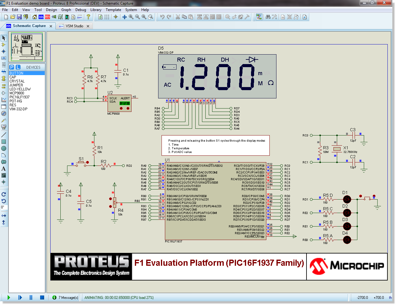
Starting from the basics of driving the simulation from the VSM Studio IDE we will then look at some of the various debugging and measurement tools available inside the Proteus VSM software.
Requirements
To work through this tutorial you will need:
- An installed copy of the Proteus Software at Version 8.0 or later. A demonstration copy of the software can be downloaded free of charge from the Labcenter website if you do not have a professional copy.
- An installed copy of the Hi-Tech PIC16 compiler at Version 9.8 or later. Download and installation of this compiler can be managed from within the Proteus software (VSM Studio IDE); we will cover the procedure for this later in the Project Setup section of the tutorial below.
We would still recommend you read through the tutorial, even if you do not have the tools installed. Most of the material - and all of the debugging techniques - are generic and will prove useful in your own designs.
Project Setup
The first thing we need to do is setup our Proteus 8 project. Since we are use a pre-drawn schematic in the form of a virtual development board this procedure is much simplified:
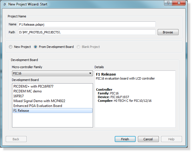
From the home page in Proteus launch the new project wizard and select the development board option. Next, change the microcontroller family to be PIC16 and finally the F1 Evaluation board (F1 Release) from the listbox at the bottom. Click finish to import the project.
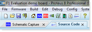
After project import you should see two tabs in the application, the schematic capture module with the F1 Release design and the VSM Studio IDE containing the standard Microchip source code for driving the hardware.
The first thing we need to do is compile the source code and produce some firmware that we can test in simulation.
Compiler Configuration
The Microchip source code was written using the Hi-Tech PIC16 compiler so we need to have this tool installed in order to compile firmware. Switch to the VSM Studio tab and launch the compilers configuration dialogue form from the Config Menu.
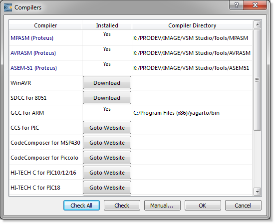
The dialogue form lists all of the supported compilers along with an indication of whether or not they are installed and configured or not. Pressing the 'Check All' button at the bottom of the dialogue will scan your computer for compilers and - if found - will configure t[hem to work directly from within Proteus.
Open source compilers can be downloaded and installed directly from Labcenter's servers. Links are provided to the download page on the vendors website for proprietary compilers The Hi-Tech compiler we need requires download from Microchip's website so if you don't have this compiler installed you will have to:
1) Click on the goto website button beside the compiler.
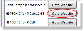
2) Download and install the compiler.
3) Click on the Check All button at the bottom of the dialogue form to configure the compiler to work with Proteus
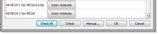
You should notice after running this command that the Hi-Tech compiler row on the dialogue form is marked as installed. The output window at the bottom of the IDE will also report on the results of the compiler checking.
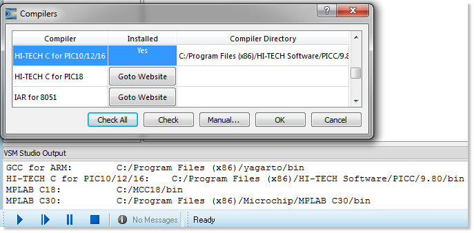
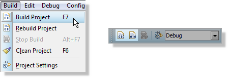
At this stage we have compiler, source code and schematic all in place. Use the Build Project command on the Build Menu in VSM Studio (or the build icon) to compile your firmware.
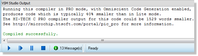
Output from the compiler is written to the bottom pane of the IDE and you should get a compiled successfully message on completion.
The next step is to run the simulation and test our compiled code on the virtual hardware.
VSM Studio automatically configures common compiler options to correctly build your programs for simulation in Proteus. If you need to tweak settings (e.g. link to external library) you can do so via Project Settings on the Build Menu.
Running a Simulation
Running a simulation is as simple as pressing the play button on the animation control panel at the bottom left of Proteus.
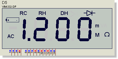
You should see that the schematic tab comes to the foreground and that the LCD panel displays the default time.
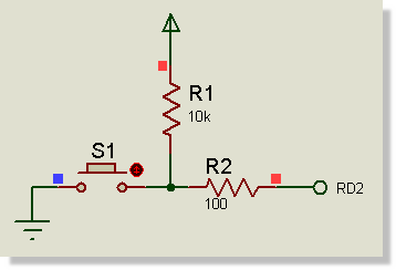
The Microchip demonstration code for the F1 Evaluation Board has three modes, one for time, one for temperature and a third which gives an ADC reading from the POT. You can interact with the simulation and cycle through the modes of operation by pressing the control button on the schematic.
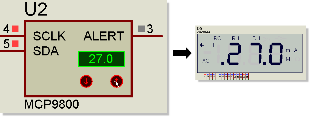
When in temperature mode you can adjust the temperature on the MCP9800 temperature sensor by clicking on the increment or decrement buttons. The current temperature is transmitted on the I2C bus to the PIC processor and then formatted and displayed on the LCD.
When in voltage mode you can adjust the value of the POT. The voltage reading is converted by the processor and then displayed on the LCD panel.
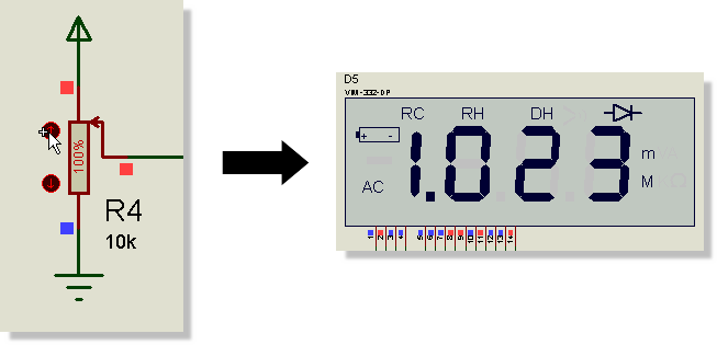
The PIC microcontroller has a 10-bit LCD so our displayed value range is 0 to 1023 over the 0 to 3.3V range.
When you are finished press the stop button on the animation control panel to stop the simulation.
Important Notes
Quite a lot is happening when we run a simulation in Proteus that might not be immediately apparent.
Firstly, the micro-controller on the schematic is executing the compiled firmware file in exactly the same way as a physical PIC would execute it's programmed firmware. Working with the VSM Studio IDE simply automates the 'programming' step by sending the output file to the schematic after a successful compile.
You will have noticed that almost all of the wires on the schematic end in a terminal with a name. For those unfamiliar with terminal connections it is worth explaining how this works. On the schematic, any two terminals with the same name are considered connected (like a 'virtual' wire). For example, the RC3 and RC4 terminals at the side of the temperature sensor correspond to the RC3 and RC4 terminals connected to the I2C pins on the PIC processor.
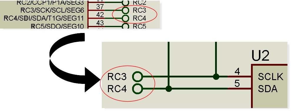
We tend to lay out schematics like this to avoid spaghetti wiring and to split the schematic into easily identifiable logical blocks. The important thing to understand is that all signals travel on the visible wires. This means that you can attach a voltage probe or measurement instrument anywhere that you can see a wire (indeed, we will do both later in the tutorial). All that ISIS does is 'jump' the signal between the two terminal ends as though there was a single wire connection. You can read up more on this type of connectivity in the ISIS reference manual.
Finally, the status bar at the bottom of the application reports the simulation time elapsed. Depending on the power of your computer, the clock speed of the processor and complexity of the schematic, a particular simulation may not run in real time but it will always run synchronously and the execution time is reported on the status bar.

As an example, on a particularly slow computer this simulation in clock mode may not advance as the clock on the wall advances but it will always advance as the simulation time advances.
Writing Firmware
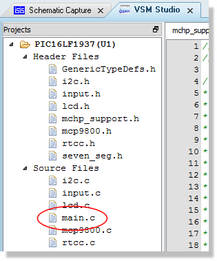
Now that we have completed the workflow through simulation let's add some functionality to the program. We know that pressing the button switches between time display, temperature and POT display so we can easily add another mode of operation here. Start by switching to the VSM Studio IDE tab and opening up the main.c file (double click on the item in the project tree).
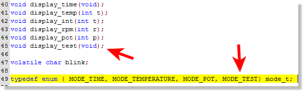
You will see near the top of the file that there are some function prototypes and an enumeration of the modes of operation. We need to add a new function prototype for our test mode and also add a corresponding value to the enum. You can add the following:
Next, we need to find the button switching logic in order to add our new mode of operation. The easiest way to do this is to search for one of the other modes. Right click on the editing window in VSM Studio, select Find from the resulting context menu and then enter MODE_POT as the search term.
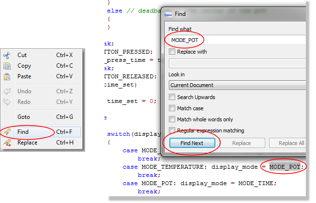
Almost the first hit is the one we are looking for, namely a switch statement on button release that cycles through the setting of the display modes. All we need do here is add our new mode.
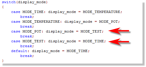
Note that you need to change the display mode on the previous case statement as well.
Just below this in the code there is another switch statement which actions the current display mode. Again, we need to our case here and call our function.
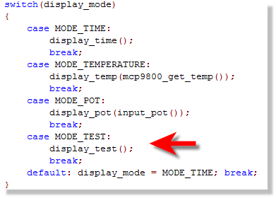
The last step is to write a function that does something when we enter our mode of operation. We'll add this at the bottom of the file.
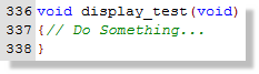
You can experiment and add anything you like here but we'll do something simple, writing a value to the display and adding a little binary counter on the LED's.
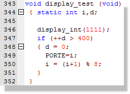
Since we are using PORTE to write the LED's here we also need to configure the port pins. We'll set up ANSELE in the peripheral config section at the top of the main function.
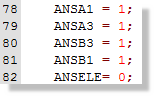
The final step is to build the project and launch ISIS as discussed before. If you have made a mistake (as we have here) you will get a compiler error in the output window. Clicking on this error will navigate to the problem. In our case we have missed a semi-colon from the end of the line.

Some errors - such as linker errors - will obviously not be navigable. In these cases you may need to change the options/includes via the project settings command.
When we run the simulation this time we can use the button to cycle through the modes of operation until our own is reached (time -> temperature -> test). We should see our displayed number on the display at this point and a byte cycle count on the LED's
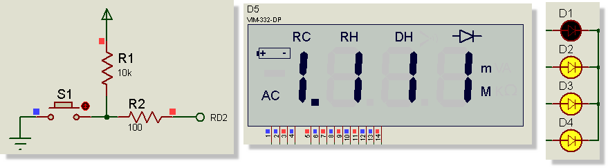
Again, press the stop button on the animation control panel to stop the simulation.
This example is a little contrived and not terribly exciting but it does show how you can quickly write and simulate code on virtual hardware.
Active Popups
So far, we have been writing our code in the VSM Studio tab and simulating on the schematic capture tab. There is nothing wrong with this and it can work very well on two monitors if you drag one of the tabs onto another screen.
When debugging however, you are typically more interested in stepping the code and looking only at small sections of the board for verification. The active popup system in Proteus is designed to do exactly that - bringing defined sections of the schematic into VSM Studio during simulation.
In our case, the temperature sensor is a good example of something we might want to see and interact with during debugging. To add it as an active popup:
1) Switch to the ISIS tab and selecting the Active Popup icon.
2) Start at the top left and drag a box around it.
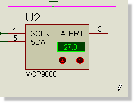
3) You should see a blue dashed line around the area when you are finished.
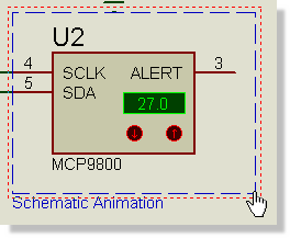
If you make a mistake you can right click on the dashed line and delete. Similarly, if your positioning is wrong, you can right click on the dashed line and drag.
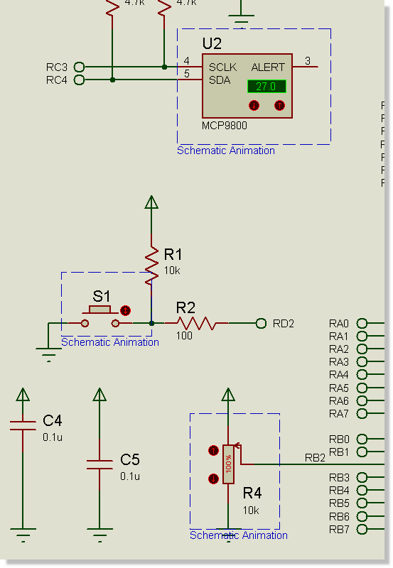
Other likely candidates for active popups are the mode selection button, the POT and the display itself so we can repeat the process above, dragging additional boxes around these items. Your schematic should look something like the following when you are finished.
Since we have specified active popups the assumption is that we will be working (debugging) inside VSM Studio. If you press the play button to run the simulation now you should find that you switch to the VSM Studio tab and that the active popups appear docked on the right hand side of the IDE.
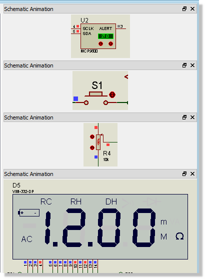
The source and variables areas of the tab will display a simulation running message at this point as we are freely executing code. We'll cover debugging in the next section of the tutorial.
Active popups are clever not only because they bring areas of the schematic into the debugging environment but because you can interact with them. For example, if you click on the S1 button to switch modes you should see the display change to the temperature on the I2C temp sensor and if you then adjust the temperature on the sensor the display should reflect the changes.
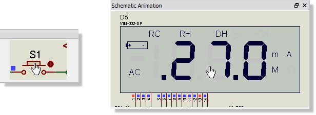
You can switch back to the schematic tab and you will see exactly the same status as in the active popups. When you stop the simulation (from the animation control panel) the active popups will disappear and VSM Studio will switch from it's 'debugging layout' to it's 'design layout' where you can once again edit and compile your source code.
You can only create or adjust active popups on the schematic when the simulation is stopped. You can however resize active popups inside VSM Studio by dragging while the simulation is running.
Now that we have configured our active popups we can start to look at how to debug problems when things don't quite work the first time.
Basic Debugging
Much of the real power of Proteus VSM comes from it's debugging capabilities. We have already seen how we can write code and test during free running simulation and we'll now look at how to step through our code in simulation time.
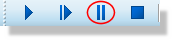
Start the simulation with the pause button on the animation control panel
The program will switch to the VSM Studio tab, active popups will display on the right hand side, the main panel will report a 'no source line message' and a list of program variables will appear at the bottom of your screen.
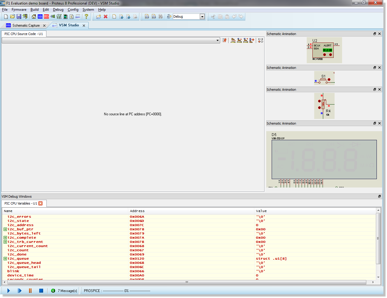
At this stage the simulation has 'booted' and a stable operating point
has been found but no instructions have executed and no real time has
elapsed.
No source code is shown as there is no source line at the current program counter value
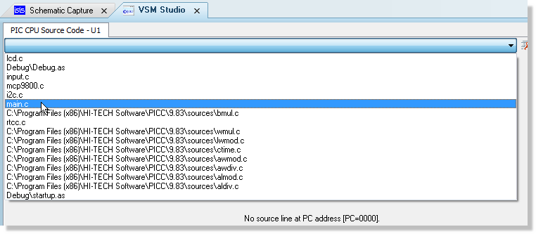
You can select any of the program source files from the combo box at the top of the window but we will start with the main.c file which contains the principle program control loop.
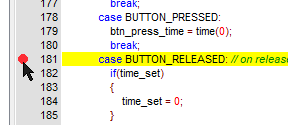
To take a simple example, lets set a breakpoint in the main event loop when a button is released. The easiest way to to set/toggle a breakpoint is to left click on the left of the line number on the line of code that you wish to break on. The breakpoint indicator should appear at the left of the source window beside the line of code in question. If you set a breakpoint by mistake then you can remove it or toggle it off by double clicking again on the line (or from the right hand context menu).
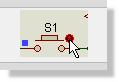
If we run the simulation now (play button) it will switch happily execute in free running mode until we release the mode switch button (S1) at which point the code for button release will be hit and the simulation will pause. You can do this easily by clicking on the button in the active popup window.
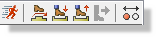
Having hit our breakpoint we can single step our code (and the system) via the usual commands which can be found at the top right of the source window or on the debug menu in VSM Studio. Alternatively you can use the F10 and F11 shortcut keys for 'step over' and 'step into' respectively.
If you really need to examine behaviour in detail you can even step the code at assembly level. Right click on the source menu and select 'disassembly' from the resulting context menu and then use the same step commands as before.
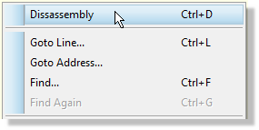
Right click and select disassembly again to return to high level source code stepping
You may notice during step debugging that the active popup for the display does not show a full legible output. This is correct and a consequence of the display being multiplexed.
If you want to run through to the next button release simply press the play button on the animation control panel and then click the button on the active popup to trigger the breakpoint again.
Right click and select clear all breakpoints when you are finished and then press the stop button on the animation control panel to end the debugging session.
Important Notes
When you hit a breakpoint or single step debug in Proteus it is important to understand that you have the entire system under time control. This means for example that capacitors will not discharge or motors lose momentum when the system is paused. When you step over a command the instructions are executed, the effect of those instructions are propagated through the system and then the system will pause again. You can see this controlled advance of time via the output on the status bar during debugging.
Many additional debugging windows are available which are not discussed in this tutorial. All of these can be launched from the debug window in VSM Studio and will appear at the bottom of the IDE. Data will be displayed on the windows whenever the simulation is paused. The watch window - which is a special case- is discussed separately in the next section of the tutorial.
The Watch Window
The watch window is the one debugging window that provides live data during free running simulation and it also gives us a different way to target breakpoints. To start with, lets use the watch window to monitor the ADC conversions from the POT.
Start the simulation using the play button at the bottom of Proteus and then launch the watch window from the debug menu in VSM Studio. You should see it appear as a docked tab at the bottom of the IDE.
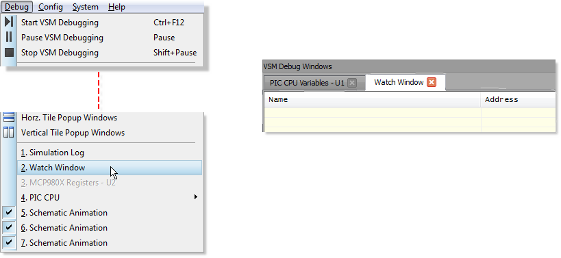
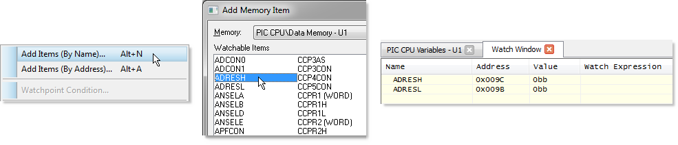
Next, right click on the watch window and select 'Add items by name' from the context menu. We want to add the ADC registers ADRESH and ADRESL which you can do by double clicking on an entry. Exit the dialogue form when you are done and you should see both items appear in the watch window display.
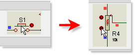
We now need to use the active popups (or switch to the schematic tab) to switch into POT reading mode. Click on the control button three times to cycle the modes and then use the actuator buttons at the left of the device to vary the value on the POT.
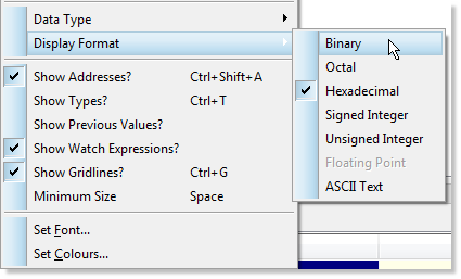
You can change the display format of the items to binary if you find it easier to understand the results. You would do this by right clicking on each item in the watch window and changing the display format to binary.
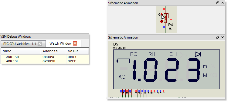
Since this is 10-bit ADC we would expect the maximum value to be 1023 or 0x03FF and we should see this value when the POT is fully ramped up.
Now lets assume that we needed to catch the midpoint on the way back down. We know that the midpoint value result should be around 0x1FF so we can set conditions on the watch items to trigger a breakpoint. We do this by right clicking on a watch item and selecting watchpoint condition from the context menu. In our case we would want to stop when both ADRESH is equal to 0x01 and when ADRESL is less than or equal to 0xFF. This will work as the first time we hit this value on the way down from the maximum will be at the midpoint voltage.
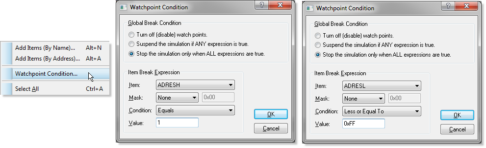
Note that you need to separately configure ADRESH and ADRESL. The watch window display should look like the following when you are finished.
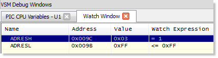
Having set up the watch conditions all we need do now is adjust the POT back down until the breakpoint kicks in when the conditions are met. As before you can do this either via the POT active popup inside VSM Studio or by switching to the schematic tab. When triggered you should see that the value on the watch items is 0x1FF and - if need be - you could start single stepping your code at exactly the point the conditions were triggered.
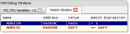
Watch conditions are particularly useful for things like debugging timer code when you want to trap an overflow condition.
You can disable watch point expressions by right clicking on a watch item, selecting watchpoint condition and then selecting the 'turn off watchpoints' option from the resulting dialogue.
Before we move on to discuss hardware breakpoints either disable the watchpoint conditions (as described above) or delete the watch items completely and then press the stop button on the animation control panel to end the simulation.
Hardware Breakpoints
So far, we have looked at how to break into the simulation based on software conditions (watchpoints and breakpoints). It is also possible to use hardware breakpoint objects in order to check the code when a hardware condition occurs. As an example, if we wanted to catch the beginning of activity on the I2C bus we could set up a hardware breakpoint on the I2C line as follows.
Switch to the schematic tab and then select the voltage probe icon from the mode selector on the left hand side. Next, click on the editing window to begin placement, move the mouse over the SDA line on the bus and left click again to drop the probe on the wire.
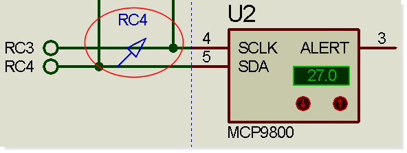
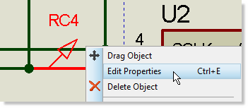
Now right click on the probe and select edit properties from the resulting context menu.
Select digital breakpoint and we want to trigger on active low so enter 0 as the trigger value.
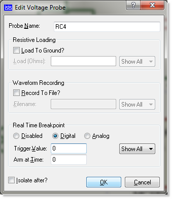
Hit OK and then press play to run the simulation. You should find that the simulation will pause almost immediately and the source window in VSM Studio will show that we have just executed a command to set SDA low.

This breakpoint is actually taking place inside the initialization routine. If we wanted to skip this and activate only when we enter I2C mode we need to set and arm time on the breakpoint. Do this by stopping the simulation, switch to the schematic module and edit as before. Set the arm time to 1 second.
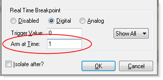
This time when we run the simulation the breakpoint will not trigger until we press the mode selection button to enter temperature mode (where temperature is transmitted on the I2C bus).
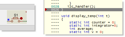
You should find that you end up inside one of the I2C routines in the source code. You can follow the code path from here using the stepping and debugging described in previous sections. Stop the simulation again when you are finished.
Interactive Measurements
It is quite common to want to examine signals and waveforms on the design and Proteus provides two main ways of doing this. As an example, let's assume we need to examine the I2C traffic from the MCP9800 temperature sensor; we can do this either interactively or by more traditional graph based methods.
The first thing we need to do is tidy up the schematic and remove the debugging items we have used previously. You can remove the voltage probe by right clicking on the probe on the schematic and selecting delete from the context menu. Similarly, we can right click on the border of the active popup objects and delete them.

When an active popup is defined on the schematic Proteus will switch to VSM Studio when the simulation starts as it is assumed you are primarily debugging source code. Since we are now analysing signals we want to remove the active popups so that the simulation starts with the schematic tab open.
The next thing to do is to get the I2C debugger placed and connected. Select the instrument icon which produces a list of available interactive measurement tools in the parts bin. In our case, the obvious candidate is the I2C protocol analyser.
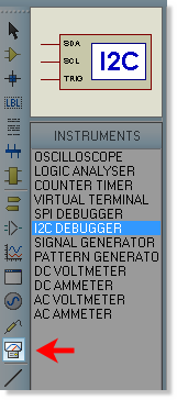
Click on the I2C analyser in the parts bin to select it and then place it on the schematic in the usual way. For ease of wiring, you'll want to drop it underneath the temperature sensor.
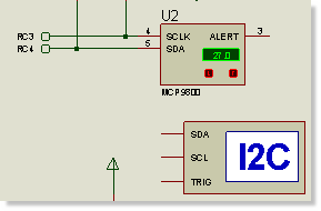
Next, we need to wire up the pins. Note that the cursor turns green on both a starting and stopping point for a wire. The wiring procedure is therefore to position the mouse over the starting point (the pin on the I2C debugger) until the cursor turns green, left click to start placement, move mouse to destination point (cursor turns green) and finally left click to terminate placement. Use this technique to connect both the SCL and the SDA lines to the I2C bus.
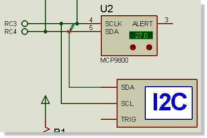
Once we have wired up the analyser we can start the simulation. You should see straight away that there is an additional window for the I2C debugger and what seems to be some initialization/identification traffic. To view normal transmission we need to press the button on the schematic to switch into temperature mode display.
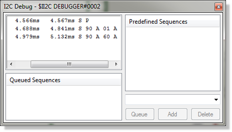
Since the code is constantly polling you should then pause the simulation from the animation control panel so that we can take some time to analyse the traffic.
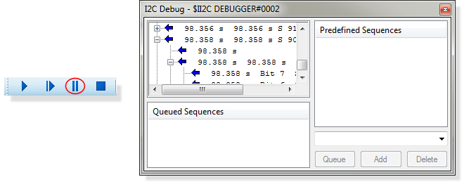
If you are working within a single frame the VSM Studio tab will come to the foreground when the simulation is paused as it is assumed you are interested in the source code pending execution. The analyser will however remain on top. If you want to see both the schematic and the source at the same time you can either use Active popups or drag the VSM Studio tab onto some free space to separate it.
The syntax used in the protocol analyser is standard and should be familiar. You can expand any sequence via the '+' box on the left hand side. The peripheral (MCP9800) has a standard address of 0x90 so we can see from the read requests that the sequence is start (S), followed by read request 0x91 (Read request, bit 0 set), followed by 0x1B (data) and so on. As you would expect the data received (0x1B) is 27 decimal corresponding to the temperature currently displayed on the peripheral.
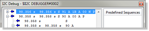
You can experiment with this by running the simulation, changing the temperature on the MCP9800 schematic part and then pausing again to check the display output on the I2C debugger.
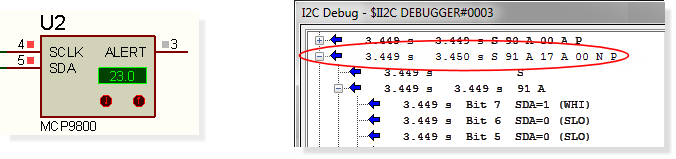
Do note that with constantly polling firmware such as this there is considerable overhead in terms of performance as we are constantly writing textual data to the display. However, in most cases you are using the instrument for testing or debugging, at which point the simulation speed is secondary to problem solving. As with all debugging windows you can close the debugger when not in use and then re-open it from the Debug Menu in either VSM Studio or ISIS.
Further Reading:
More information on the protocol analyser - along with other instrumentation - is available in the Proteus VSM reference manual. In particular, note that you can use the analyser as an I2C master (or slave) device as well as simply as a monitor.
More information on picking, placing and wiring on the schematic can be found in the ISIS tutorial documentation, launchable from the home page.
Graph Based Measurements
We can look at the same traffic in a different way by using graph based simulation. There are however some important differences which affect how we set up the simulation, namely:
- You cannot interact with the circuit during a graph based simulation.
- A graph based simulation runs for a specified period of time.
- The results are not visible until this period of time has finished and the simulation has stopped.
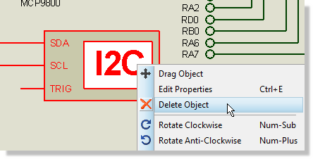
Given the above, let's look at how we might analyse the I2C traffic with a digital graph. First of all, delete the interactive I2C debugger by right clicking on it and selecting delete from the context menu.
Next, make some space for the graph by dragging a tagbox around the display and wires with the right mouse button so that they all highlight. Left depress the mouse and drag the lot to the right of the schematic.
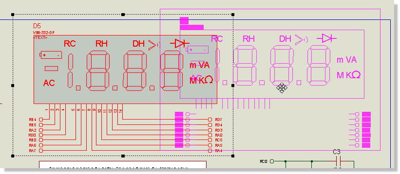
Now select the graph icon and then the digital graph from the parts bin. Left click the mouse at the top left of where you want the graph to be and then move the mouse down and to the right. Left click again to commit placement.
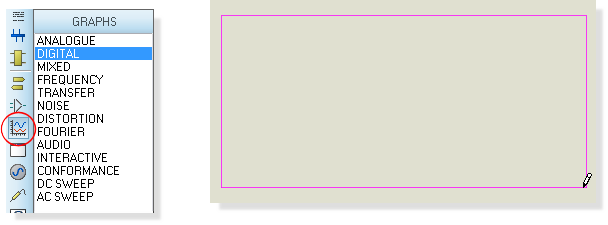
Note that the graph on the schematic doesn't need to be particularly large. We will maximise it later when we want to analyse the simulation results.
Having added the graph we now need to tell it which wires we want to trace. We do this by attaching probes to the wires and then specifying the probes as traces on the graph. Select the voltage probe icon and then place a probe on each of the two I2C lines. This is done exactly as we discussed earlier in the section on hardware breakpoints.
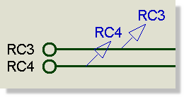
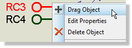
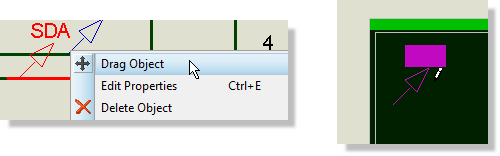
If you need to make some room for the probes, right click on the terminal at the end of the wire, right click and select drag object from the context menu and move to the left to make room for the probe.
You can use the middle mouse button or the F6/F7 keys to zoom in and out around the mouse position if you need to get in closer. The F8 key will return to the default view of the schematic.
By default, the voltage probes will pick up the name of the terminal. Its useful to rename them to be more meaningful in the context of our simulation. You can do this by right clicking on the probe, editing it's properties and then changing the name to be SCL or SDA respectively.

Now that we have the probes on the wires and the graph on the schematic we need to add the probes to the graph. There are several ways to do this but probably the easiest is simply to drag the probe onto the graph. To do this, right click on the probe, select drag object, move the mouse over the graph and then left click again to drop. Do this for both probes.
By default, a graph based simulation will run from time zero to one second of simulation time. In our case, it would make much more sense to run from one second to two seconds, thus skipping the initialization traffic. We can do this by editing the graph (right click and edit properties) and changing the start and stop time.
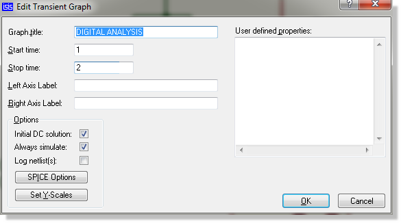
Left clicking on an empty area of the schematic will de-select any currently selected objects. Normally, this is done when you exit an edit properties dialogue form as the object will still be highlighted.
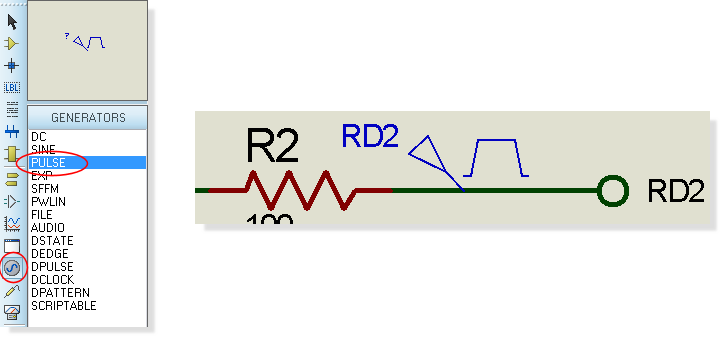
We are now ready to simulate except for one significant problem. As mentioned previously, you cannot interact with a circuit during a graph based simulation but we need to switch mode in order to poll the temperature sensor and trigger the I2C traffic. Since we can't press the button we need to inject an equivalent signal to the PIC so that the firmware switches into temperature mode. We do this with generators. Select the generator icon and then the pulse generator from the parts bin. Place the generator to the right of the button beside the RD2 terminal - you may need to move the terminal first to make some space on the wire for the generator.
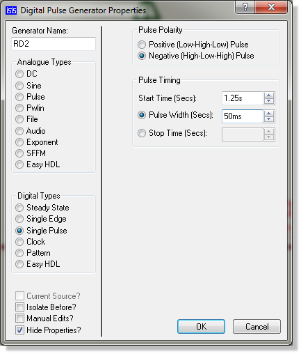
Now edit the generator in the usual way (right click - edit properties). Select single pulse from the digital generator types and change the pulse polarity to be negative so that the pulse signal represents a button push. Since we are simulating from 1s to 2s set the start time to 1.25s and the pulse width to something like 50ms.
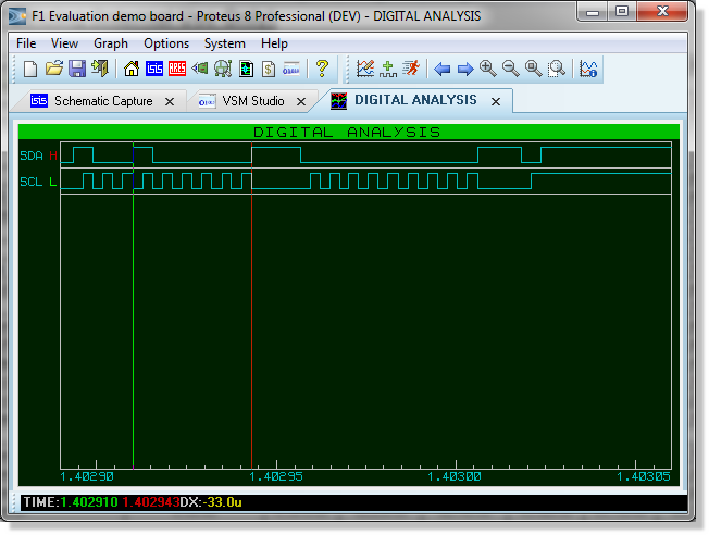
We can now run the simulation. Unlike an interactive simulation the animation control panel is not used (we are simulating for a fixed time which does not necessarily start at time zero). Instead, use the 'Simulate Graph' command on the graph menu. You should then see results which look like those below.

Aside from the fact that the traffic didn't start until around 1.25s (as specified by the pulse) we can't see much information here. Right click on the graph and select maximise from the context menu to launch the program in a new tab.

When the graph tab is in the foreground the menu's and icons change to show things we can do with the graph. In particular, notice the new graph toolbar at the top of the application

The zoom commands can be found here and probably the most useful of these is the 'zoom to area' icon. Click on this icon and then drag around a small area to localise the display. If you repeat this you will soon be able to zoom in on a single I2C sequence.

Alternatively, you can hold the SHIFT button down and drag a box with the mouse to zoom into the area inside the box.
Those familiar with the I2C protocol can then verify the raw data on the graph against the sequencing we saw earlier on the protocol analyser.
Finally, you can take measurements with the graph as follows:
- Left clicking the mouse on the graph window will place a (green) cursor on the graph.
- Left dragging the mouse will allows you to position the cursor
- Holding the CTRL key down and left clicking will place a (red) cursor.
- Left dragging the mouse with the CTRL key down will allow you to position the (red) cursor.
- Data for each cursor and delta between them is shown on the display at the bottom of the graph window.
Further Reading
All of the general placement and editing techniques discussed briefly here are covered in far more detail in the ISIS tutorial documentation.
More information on Graphing is provided later in this documentation and a full discussion of generators, probes and graph based simulation can be found in the Proteus VSM reference manual.
Diagnostic Messaging
Another - often overlooked - tool provided in Proteus is diagnostic messaging. This is an interface that allows you to ask the system for a plain text report of activity in a particular peripheral or peripherals. To look at this we will turn on diagnostic messaging for the LCD panel.
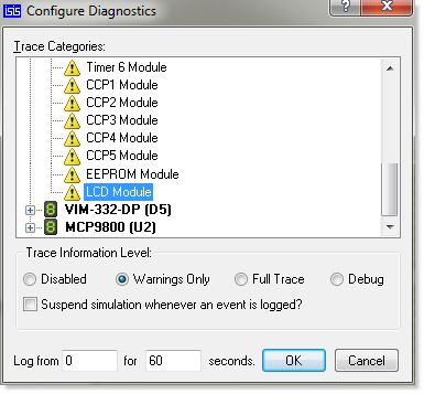
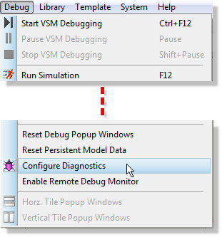
Switch to the schematic tab and then launch the configure diagnostics command from the Debug menu.
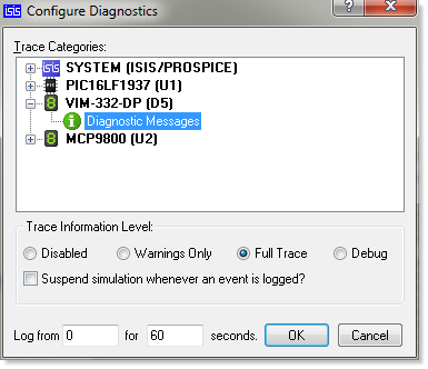
Expand the entry for the display panel, click on the entry and then change the trace information level to full trace.
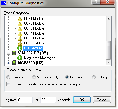
Now expand the PIC16 and scroll down to the LCD module entry, again changing the trace information level to 'full trace'.
Start an interactive simulation from the animation control panel and then click on the simulation advisor to view the diagnostic messages. This will switch Proteus to the VSM Studio tab and the simulation advisor will appear as a docked window at the bottom of the frame.
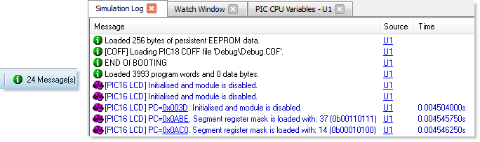
If you pause the simulation note that the LCD messages contain PC values which you can click on to locate the instruction in your source code that caused the condition.
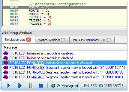
Navigation to source code is only possible when the simulation is paused.
Finally, stop the simulation and turn off diagnostics in the same as they were enabled, except change the trace information levels back to warnings only.
Diagnostic messages are particularly useful in a problem situation where you need to gather information before deciding where to hunt for the bug. It does generate a major performance hit (try it with the PIC MSSP peripheral and MCP9800 in temperature mode for example) and should therefore only be enabled when required. You can also choose to log over only a limited time period if you know when the activity band of interest is.