FINISHING UP
Power Planes
You can load the "IoT Pump - Routed" sample design in order to continue from this point, if you have not already successfully completed the previous sections.
Power Planes (also called "Zones", "Copper Pours" and "Ground Planes") are areas of the board which are filled in with copper, and usually connected to some power net (such as Ground or VCC). They can serve a number of purposes, including:
- Providing a reference plane for impedance-controlled traces (high-speed tracks, differential pairs, RF tracks, etc).
- Reducing EMI/EMC.
- Satisfying requirements for wireless module antennas.
- Reducing manufacturing costs.
- Providing low-impedance paths for power to travel along.
- Adjacent power planes on different layers can be used to form a capacitor, which can be used to smooth high-frequency power fluctuations.
PCB Design Level 2 and up allow an unlimited number of shape-based power planes per layer. Lower PCB Design levels only allow 1 power plane per layer, which must cover the entire board.
There are a number of options for creating power planes and we will explore a few of these.
The most simple option is the Power Plane Generator which is available from the Tools menu.
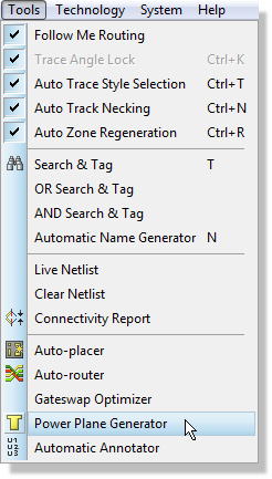
Opening the Power Plane Generator from the Tools menu
From the resulting dialogue form select the GND=POWER net, and set the layer as top copper with the DEFAULT boundary style. The boundary style determines the trace which will be used to draw the inner and outer boundaries of the zone and also determines the thinnest section of copper by which the power plane can make a connection. Setting the boundary to a thicker track style will prevent the copper flowing through small gaps (e.g. between pins) but making it smaller means that connectivity may be achieved even by only thin sections of copper.
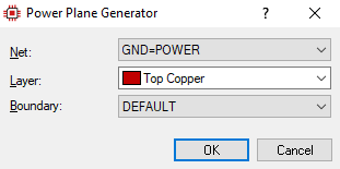
Power Plane Generator Dialogue Form
Click "OK" and you should see that the power plane is generated on the Top Copper layer across the entire board.
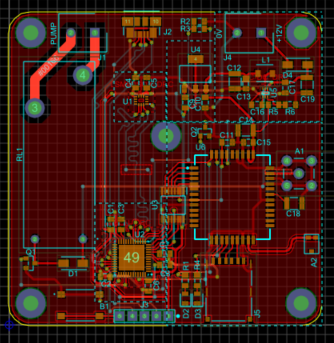
Power Plane has flooded the entire layer
The clearance from the zone to the board edge is defined by the Edge/Slot design rule. We can change this via the Design Rule Manager on the Technology and the zone will re-generate to the new clearance when we have finished.
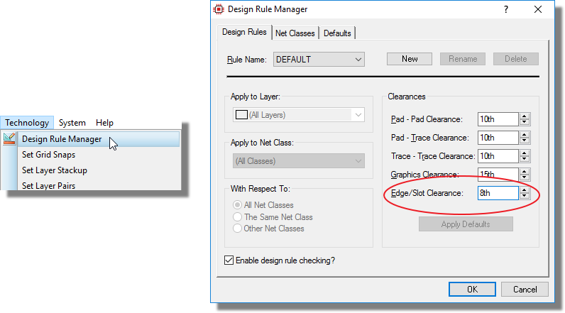
Since you can set a new design rule per layer it is possible to have different clearance rules for power planes on different layers.
The next option for generating a power plane is from the Layer Stackup and Drill Spans dialogue (we could actually have done this during the New Project Wizard when starting the project). Launch the dialogue by selecting "Set Layer Stackup" from the Technology menu. Select the Bottom Copper layer and then click "Create Power Plane". Select net GND=POWER and then click OK to generate the plane.
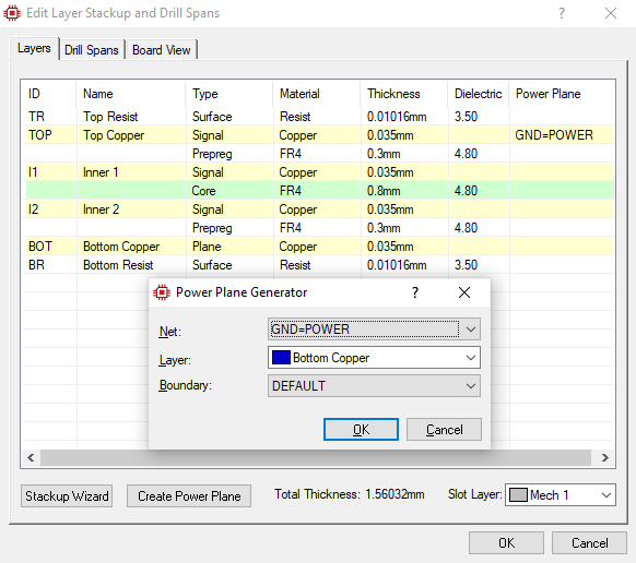
Creating a power plane from the Layer Stackup and Drill Spans dialogue
Create a GND=POWER plane on the Inner 2 layer as well, and a VCC/VDD=POWER plane on the Inner 1 layer.
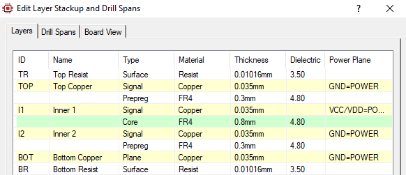
Power planes on all layers
The third option for creating planes, and also the most flexible, is using the Zone mode - we will look at this a little later.
Nesting and Islands
There are several additional configuration options available to us now that we have placed some zones. Editing a zone is slightly different from most other objects in that you must right-click on the border of the zone (to avoid continuous unwanted selections).
Firstly, check the selection filter to make sure that the zone object type is selectable (or switch to selection mode).

Zone icon in the Selection Filter
Next, zoom in and move the mouse over the edge of the zone, right clicking the mouse when the zone is shown as active under the mouse. Select Edit Properties from the resulting context menu.
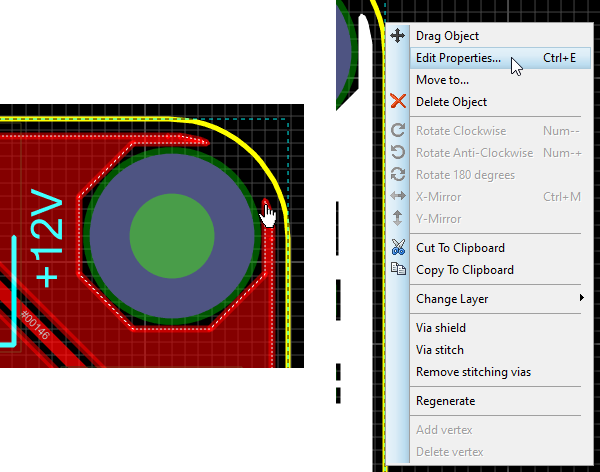
Right click on the edge of a zone to edit its options
The main options of interest are towards the bottom of the dialogue form and are explained below:
Relieve Pins
When checked then pins on the same net as the zone will have thermal relief applied to them; the thickness of the thermal relief is determined by the Relief field of the dialogue form.
The software will prevent you from using a relief track style that is larger than the boundary style thickness; this is to protect against the reliefs 'sticking out' of the boundary.
The topology of the relief stems on a particular pad can be changed to a diagonal 'X' by editing the pad itself after placement. This is sometimes useful to maximise contact with a zone.
This option should almost always be left in it’s default checked state.
Exclude Tracking
If this option is checked, the zone will treat tracks on its own net as obstacles. Otherwise the zone flows over such tracking, effectively ignoring it. Tracks on other nets, or loose pieces of track on no net are always treated as obstacles.
This option is normally left unchecked.
Suppress Islands
An island is defined as a block of copper or zone area in which no valid connections can be made. When checked, Proteus will remove all such blocks from the board, leaving only areas of copper with connections.
Allow Nesting
It is quite common, particularly with larger boards, that the flow of a zone will encounter an obstacle through which it cannot pass. When checked, the zone will jump over the obstacle and continue flowing across the board.
This is a very useful option for example on busy boards or where you want to connect a pad where the topology of the board makes it impossible for a single zone flow to get through.
The default options are fine for our purposes, however you may wish to experiment a little with the various options in order to see how they work (make sure to "Undo" again afterwards).
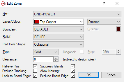
Edit Zone dialogue
Zone Exclusions
Sometimes there is a need to exclude a plane from a certain section of the board. This can be done by placing an "empty" zone within that plane. In our case, we should create an "empty" zone around the BlueTooth antenna. Start by selecting "Zone Mode" from the mode bar.
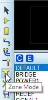
Zone mode
Draw a rectangle around the BlueTooth antenna as shown by clicking at each of its four corners.
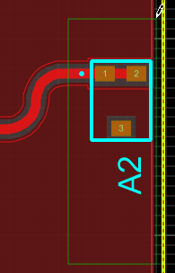
Drawing a zone
Once the zone shape has been closed then the "Edit Zone" dialogue will appear.
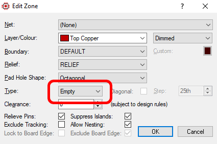
"Empty" zone type
Set the zone layer to Top Copper and the zone type to "Empty" and then click OK. You should then see that an exclusion has been created in the Top Copper power plane, around the BlueTooth antenna.
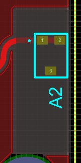
Zone exclusion placed
We now need to recreate this exclusion for the zones on the remaining 3 power planes / layers. We could draw the zone over again 3 times, selecting a different layer each time, however it will be easier to simply copy the zone. In Selection mode (cursor icon), draw a box around the zone.
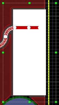
Selection box around zone
Unless you have changed the selection filters, everything within the box will now be selected (including the track and the BlueTooth antenna). In order to select ONLY the zone, so that we can copy it, we can use the Selection Filters to target only the zone.

Only the "Zone" selection filter toggled on
We can now use the Block Copy tool to make a copy of the zone over to the right of the board.

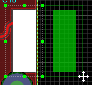
Block Copy the zone over to the right
Go into the zone properties and change it to apply to the Inner 1 layer.
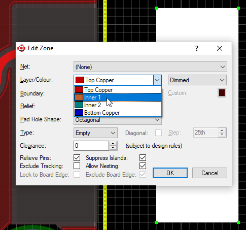
Change the zone to apply to the Inner 1 layer only
Next drag the zone back over to the left, to coincide with the Top Copper exclusion zone.
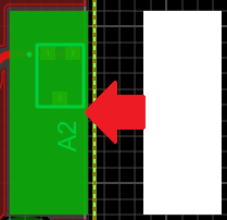
Dragging the zone back
We now have exclusions on both the Top Copper and Inner 1 layers, and we simply need to repeat the process for the Inner 2 and Bottom Copper layers. Note that if selecting and block copying again then we will now be copying over two exclusion zones (Top Copper and Inner 1) - this is fine if it is intentional and we plan to change these two zones to be Inner 2 and Bottom Copper; but the alternative is to set the Selection Filter to target only the currently selected layer, so that we only copy over one zone at a time. Use whichever method you prefer to place exclusion zones on the remaining layers.

Filter the selection to the current layer only
Once done you should now see that all planes are clear of the BlueTooth antenna area.
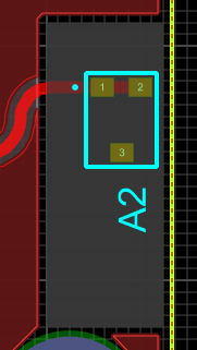
Zone exclusion present on all layers
See Also:
Power Planes Examples (Reference Manual)
Using Power Planes (Reference Manual)
Plane Layers (Reference Manual)
Zone Inspector (Reference Manual)
Via Stitching and Shielding
Via Stitching and Shielding can be used to stitch power planes together with vias, for EMI/EMC / RF / etc reasons. Vias can be arrayed:
- Throughout the area of a plane, in a grid fashion (stitching).
- Around the edge of a plane (shielding).
- Along the length of a track (shielding).
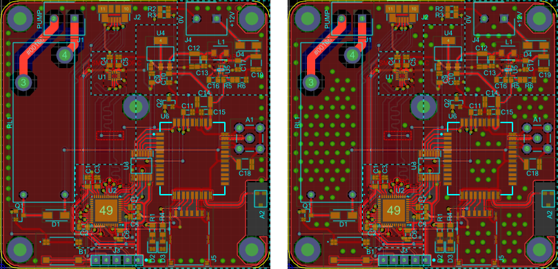
Via Shielding and Via Stitching
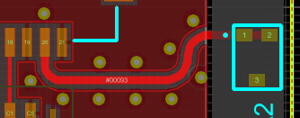
Via Shielding a Track
To apply via stitching / shielding between planes, select the relevant option from the plane or track right-click context menu (remember to right-click click on the edge of a plane in order to access its context menu).

Stitching and shielding commands on the Zone and Track context menus
Let's apply some shielding along our BlueTooth antenna trace. Right click on the trace and select "Via shield" from the context menu.
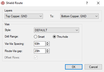
Stitching and shielding commands on the Zone and Track context menus
Set the vias to go from the Top Copper layer to the Bottom Copper layer; style "Default"; via-via spacing 60th and route-via gap 20th. Click OK once done and you should see that vias are placed along the length of the BlueTooth Antenna track.
Shielding along the BlueTooth Antenna track
You may wish to experiment a little further with the via stitching / shielding tools. Once done,be sure to undo any changes before proceeding with this tutorial.
See Also:
Via Stitching and Via Shielding of Power Planes
Zone Regeneration
By default, zones are automatically regenerated whenever any changes are made to the board. Zone regeneration takes some processing power, so if you find that this is slowing you down then you can turn off automatic zone regeneration, either temporarily or permanently; zones can be manually regenerated from their right-click context menu.
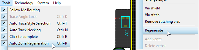
Automatic and manual zone regeneration
Slots and Cutouts
Sometimes there is a need to create slots or a cutouts in a board. We may wish to slot a board to provide additional electrical insulation as an example, and we may wish to create a cutout to allow a connector to pass through as another example. We don't actually need any slots or cutouts on this particular board, but let's experiment a little to become familiar with the functionality.
Select 2D Line mode, the Slot layer, and then draw a slot between the relay connector pins and tracks. You will need to draw two line segments to match the following screenshot, and may need to move the relay tracks slightly.
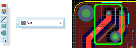
Drawing a slot
To make the slot a little thicker, hold down the CTRL key and click once on each slot segment to select them both.
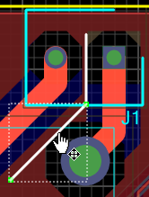
Selected items are white
Right click on any line and select Edit Properties from the resulting context menu.
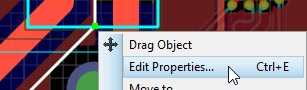
Switch to the "Edit Style" tab, uncheck the Follow Global checkbox, change the width to be 50th and then apply to all tagged graphics.
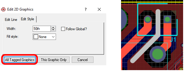
Changing multiple objects at once
To create a cutout, could either use a closed slot or we could select the Board Edge layer and draw any closed shape on the board. Let's experiment with a triangular-shaped cutout at the bottom-right of the board.
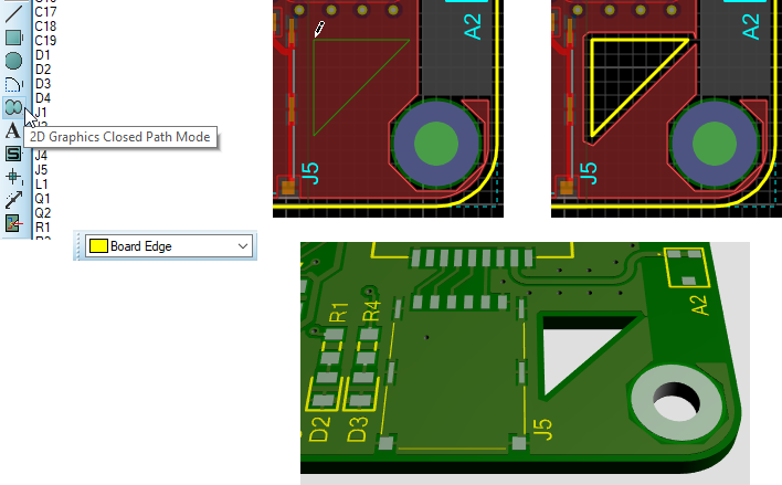
Creating a cutout
Once done experimenting, you can delete the slot / cutout.
Fiducials
Fiducials are used by automated assembly equipment, such as pick-and-place machines, to precisely locate the position of the board. To place fiducials, select Circular SMT Pad Mode, select the "FIDUCIAL" type pad, and then click on the board to place the fiducial(s).
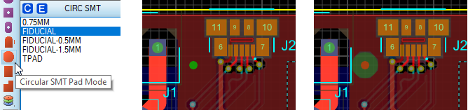
Placing a Fiducial
Fiducials can be including in Pick-and-Place output files as well as listed in the report module (more on these to follow). Usually at least two fiducials are required, at diagonally opposite ends of the board, so place at least one more fidcual on the board at the diagonally opposite corner.
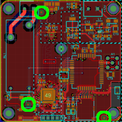
Board Fiducials
Text and Graphics
The Top Silk layer of our board already contains a lot of information in the form of component references and outlines.
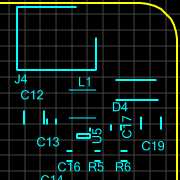
Elements on the Top Silk layer
If we would like to add additional elements then this can easily be done using the various 2D graphics tools. Typically additional text / graphics would be placed on the Top Silk or Bottom Silk layer, but elements could be placed on any of the copper layers or even the Solder Resist layers and so on if desired. You could even have more than one silk layer per side, usually with different colours, by placing elements on one of the Mech layers in Proteus and then instructing your PCB manufacturer that these should be additional silk layers (you may have both white and black silk prints on your board, for example).
Let's place some board name and version text on the Top Silk on an open area of the board. Select the 2D Graphics Text tool, select the Top Silk layer, and click in an open area of the board.
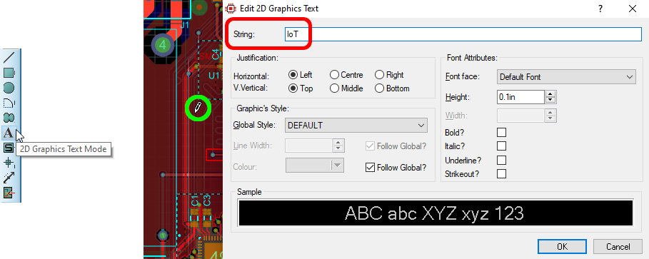
Placing 2D Graphics Text
Enter "IoT" as the String. There are a lot of customisations available (of particular note are the "Justification" options), however the default settings should be fine for us so just click OK.
Add more lines in order to make up the text "IoT Pump Controller". The last line will be a version line, and we will use a special trick here to have the label text automatically update whenever the board version (as set in the schematic Design Properties, available from the Design menu) is changed - enter "@Rev" as the string and the board version will automatically be filled in.
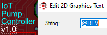
Using a variable in 2D Graphics Text
We can also import bitmaps (must be monochrome) and DXF drawings. You may wish to import the board outline from a DXF, for example. In the following screenshot, a bitmap of the Proteus logo has been imported onto the Top Silk layer of the board. The logo is in the IoT_Pump_Resources subdirectory of the Proteus Tutorials sample directory (typically "C:\ProgramData\Labcenter Electronics\Proteus 9 Professional\SAMPLES\Tutorials") if you would like to try this yourself.
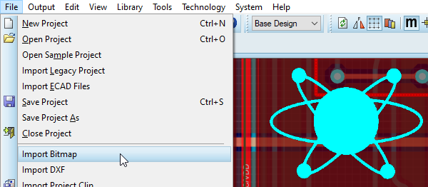
Bitmap import
Let's also place a "Pin 1" marker by the ICSP connector. Select the 2D Graphics circle tool and draw the circle next to pin 1 of the connector, then edit the circle properties and set the fill style to "Solid".
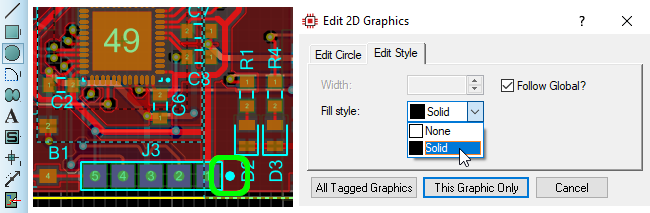
2D Graphics Filled Circle
Finally, place some labels next to the terminal connectors (rotate as necessary).

2D Graphics Filled Circle
Netlists and Design Changes
We have now placed and routed our layout based on the schematic we designed in the tutorial. In practice however, it is very unlikely that we would not be making design changes during the PCB process so we'll devote a little time to examining a typical workflow.
Clearly, we will be editing both the schematic and the layout modules so both need to be open. If the schematic tab is closed you can open it from the application module toolbar at the top of the Proteus application.
Schematic module icon on the Application toolbar
Since we will be working with both modules you may want to split them into two frames if you have two monitors. To do this simply drag one of the tabs onto the other monitor. For this documentation, we will assume that both the schematic and the layout are open as tabs inside a single Proteus frame.
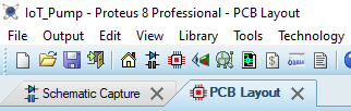
Multiple tabs in one frame
Live Netlisting
First, lets delete the J3 connector on the schematic. Switch to the schematic tab, right click and select delete object from the resulting context menu.
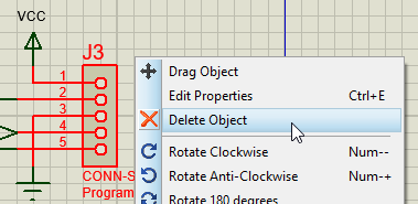
Deleting a component on the schematic
Now switch back to the PCB tab. Note that the J3 part has been dimmed to show that it is not present on the schematic and that the connectivity status shows that we have pending changes (we are out of sync).
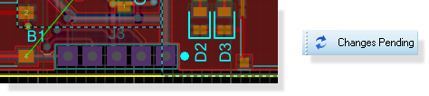
Netlist is out of sync
Since the action taken on the schematic removes from the board it requires manual confirmation. We can now either hit undo (CTRL+Z) if we don't like the change or we can click on 'Changes Pending' in the connectivity status to accept the change. When we do this, we'll be presented with a short dialogue to either show all the changes (sometimes not obvious on a dense board) or to simply commit the changes.
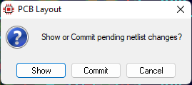
Since it's clear what the change is in this case we can simple commit the change and the 'shadow' part will disappear.
Clicking on Changes Pending will remove J2 and correct the netlist
Note that tracks that were connected will also be deleted. If you want instead to delete only the footprint (leaving the connected tracks in place as stubs) then you can do so by directly deleting the package on the layout.
The undo system is still available to revert the changes. Clicking on the UNDO icon (or CTRL+Z) once will bring back the shadow objects and repeating the process a second time will bring back the schematic part and the real PCB footprint.

Undo and Redo icons
If you click on undo while in the layout tab but the undo action applies to the schematic you will be prompted to confirm the operation. In our case, we do want to bring back the connector so accept the prompt to return the PCB to the original state.
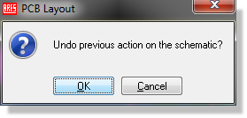
This is a simple example of a change which affects objects already placed on the layout. The important thing to remember is that while the netlist is live, you must manually confirm any change which affects the connectivity of objects you have already placed.
Batch Netlisting
If you prefer, live netlisting can be turned off and a more traditional batch mode netlist used. This is controlled from the 'live netlist' toggle on the Tools menu (in the PCB module).
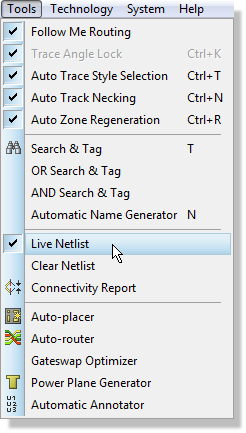
Having turned live netlisting off, let's repeat the same procedure to see the difference. Switch to the schematic tab, delete the connector and then switch back to the PCB tab. This time the connector on the PCB remains present and the connectivity status reports that the layout is locked and out of sync.
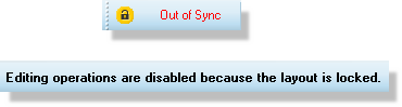
Status bar messages when 'out of sync'
This means that we have not loaded the changed netlist and cannot work on the layout until we bring the netlist across. Proteus works with a single database of parts that include schematic components and pcb footprints so - while you can work on the schematic - you cannot work on the PCB until you sync it with the schematic. Click on the connectivity status to unlock the PCB and bring the current netlist across.
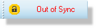
This brings us to the same state as we arrived at automatically with live netlisting on. We have a shadow part in Proteus and the connectivity status reports changes pending.
The main difference between live netlisting and batch netlisting is only that you must confirm each netlist load manually in the latter mode. We recommend that live netlisting is used for normal working, although for particularly large designs batch mode may provide a useful tool.
Some functionality will require a live netlist and so if you are working in batch mode you may find menu commands disabled until such time as you bring the netlist back in and sync.
See Also:
Netlist Features (Reference Manual)
Annotation
Annotation changes from schematic to layout or from layout to schematic are also a common editing operation when both modules are in use.
Schematic to PCB
Annotation changes made in the schematic will automatically be reflected in the PCB when live netlisting is on and will require unlocking when live netlisting is off. The Global Annotator on the Tools Menu on the schematic can automate this task.
PCB to Schematic
You can re-annotate the board either manually (editing the part reference labels) or globally from the automatic annotator command on the tools menu.
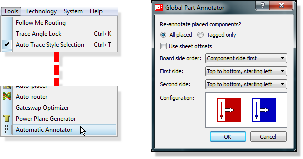
Launching the Automatic Annotator
When live netlisting is on, this will automatically reflect to the schematic. With live netlisting off, the schematic will update and the layout will then lock as the netlist has changed and needs to be manually passed through to the layout.
General Netlisting Rules
There are several important rules of thumb to understand about netlisting in Proteus.
When live netlisting is on, a change that adds connectivity will happen automatically (e.g. adding a wire on the schematic will add a ratsnest on the layout). If you make a change that removes connectivity the layout will show the change by dimming the deleted objects and you will need to manual confirm the operation.
When live netlisting is off (batch netlisting) any and all changes to the netlist will require you to unlock and apply the netlist before you can continue working on the layout.
Clicking on changes pending to remove footprints that have been deleted on the schematic will also remove associated tracks. If you want to remove footprint only and leave the tracks simply delete the part on the layout (rather than the schematic).
Dimmed objects are visual placeholders only - they do not exist on the board. Best practice is always to click on changes pending on the connectivity status and to arrange the layout to conform to the schematic.
Imported projects (from older versions) will always start with live netlisting off as there is no way to tell whether they are in sync. By contrast, new projects will always start with live netlisting on. In either case you can switch according to preference from the live netlisting toggle on the Tools menu in the PCB layout module.
3D Visualisation
Now that the board is routed and ready for production we first want to examine it in 3D in order to properly preview how it will look in real life and possibly make final design alterations prior to prototyping. Start by invoking the 3D Visualisation Engine from the module toolbar at the top of the application

3D Viewer icon
This will open and load the 3D view of the board in a separate tab. As with any tab, you can drag onto a separate frame if you want to look at both the 2D layout and the 3D view simultaneously.
Basic Navigation
The first thing we can do is view the board from different preset angles. Five preset views are supplied: top view, front view, back view, left view and right view and these are accessible via any of the following methods:
- Menu options on the View menu in the 3D Viewer
- From the navigation toolbar at the bottom of the 3D Viewer
- From keyboard shortcuts F8 through F12 whilst in the 3D Viewer.
Now that we can look at the board from a number of angles the next thing is to be able to look at it at a specific zoom level. Again, there are numerous ways to zoom in and out of the board:
- Roll the middle mouse wheel in and out (recommended)
- Menu options on the View menu
- From the icons on the Navigation Menu
- From keyboard shortcuts F6 (zoom in) and F7 (zoom out)
Experiment now with custom zoom levels and different preset views – whilst it is pretty subjective we envisage most users changing views via the navigation toolbar or keyboard shortcuts and using the middle mouse wheel to zoom in and out.
Bareboard View and Height Clearances
For inspection of resist and hole depth it is often useful to view the board without components. Selecting the bareboard view will remove all the physical components from the board.

Show Components icon
By contrast, if you need to fit the PCB into a chassis and wish to check height clearances you can enable the height boundary box via the icon at the bottom of the display

Casing icon
Specification of the height takes place from the Dimensions command on the Template menu of the viewer. This will default to the values defined in the layer stackup.
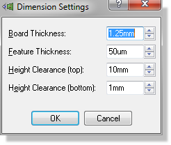
Board properties dialogue form
Custom Views
The next logical step is to be able to customise the view. This works conceptually by ‘attaching’ the mouse to the camera such that as you move the mouse the camera moves to the area of the board that you are interested in. You can invoke the Navigation mode either from the View menu, the crosshairs icon on the Navigation toolbar or simply by clicking the left mouse button.
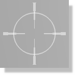
3D Mouse cursor
You will know as soon as you are in Navigation mode as a crosshair cursor will appear over the mouse and your view of the board will change as you move the mouse. Using this together with the middle mouse wheel zoom will allow you to both ‘fly pass’ the board and to easily zoom in to closely examine a particular area of the board. Exiting navigation mode is as simple as right clicking the mouse.
For example, if we start in Front View (use the F9 keyboard shortcut) and we want to examine the resistors on the right we might proceed as follows:
1) Left click the mouse to enter navigation mode.
2) Move the mouse over the resistors.
3) Roll the middle mouse button to zoom in as required.
4) Right click the mouse to exit navigation mode.
The final necessary piece to completely customise the view is to allow users to spin or ‘orbit’ the board. This is done in navigation mode by holding down the left mouse button and moving the mouse. Essentially this will spin the board as you move the mouse – when you release the mouse button the camera will follow the mouse around the current view of the board as normal. Try this now, experimenting with different views of components on the board.
Remember that, if you are struggling to get the view you want you can use the keyboard shortcuts or navigation toolbar to return to one of the preset views. You should find however, that with only a little practise you become quite proficient at navigation.
To summarise:
- Left click enters navigation mode.
- Camera follows mouse around the board in navigation mode.
- Using the middle mouse wheel (or shortcut keys) allows you to zoom as you move the camera.
- Left depressing the mouse in navigation mode allows you to spin/orbit the entire board.
- Right click of the mouse exits navigation mode.
3D Models (STEP/IGES)
Each footprint on the layout can also have an associated 3D model. Normally, these are either STEP Files (for large or complex parts) or scripted geometric models (for simple passives).
In the case of STEP or IGES files, the procedure is:
1) Download the file from the internet or otherwise source the 3D model. There are many sites available, with www.3dcontentcentral.com being amongst the most popular.
2) Save the file into the MCAD directory of your Proteus installation. By default, this is
C:\ProgramData\Labcenter Electronics\Proteus 9 Professional\MCAD\
3) Right click on the footprint and select 3D Models..., and then click on the 3D Mechanical Model tab.
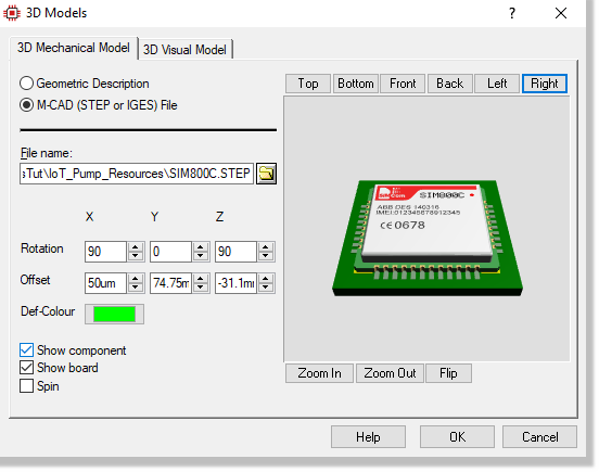
4) Browse to the STEP file and then set the rotation and offset required to align the STEP file with the pads on the board.
For geometric models, the difference is basically that you describe the part in terms of size and shape via a simple scripting language. This is covered in the reference manual.
You may notice that some components on our board are missing 3D models. You should be able to find the STEP files for any missing models in the IoT_Pump_Resources subdirectory of the Proteus Tutorials sample directory (typically "C:\ProgramData\Labcenter Electronics\Proteus 9 Professional\SAMPLES\Tutorials").
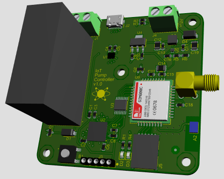
3D Visualisation of the IoT Pump Board
See Also
Live Update
Like any other module in Proteus, the 3D Viewer will update live as changes are made to the PCB layout module. In practice, the usefulness of this will depend very much on the power of your machine (number of cores, memory, etc.) and the complexity of the board.
On a board of modest complexity and a modern computer the redraw time is not significant and - particularly on split frames - is very useful for movement and positioning.
More information on 3D Visualization including creation your own 3D models, exporting 3D STEP Files for MCAD import, customizations and applying 3D data to legacy designs can be found in the 3D Viewer section in the online reference manual.
Board Output Options
Last, but by no means least, we come to the crucial business of reproducing the pretty on screen graphics on paper or film. Under Windows, most hard copy devices are supported through the normal Windows printer drivers. Additionally, we supply our own drivers for pen-plotters, Gerber photoplotters and Excellon NC drill machines.
Printing
We will deal here firstly with printing to an ordinary Windows printer device - it is unlikely that you will have a photoplotter to hand! The first step is to select the correct device to print to using the Print Layout command on the Output menu. Clicking "Configure Printer" on the top section of the Print Layout window activates the Windows common dialogue for printer device selection and configuration. The details are thus dependent on your particular version of Windows and your printer driver - consult Windows and printer driver documentation for details.
Then, with a layout loaded, invoke the Print command by clicking OK.
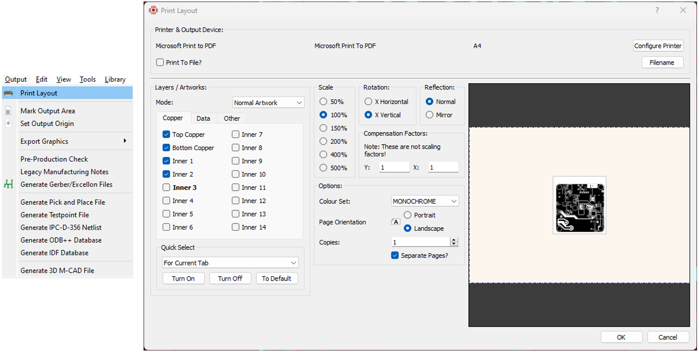
The dialogue forms offer a number of controls, all of which have detailed descriptions available when clicking on the help (?) icon on the top right of the window. The default settings should do for now. You commence output generation by clicking on OK. Output can be aborted by pressing ESC, although there may be a short delay before everything stops whilst Proteus and your printer/plotter empty their buffers.
With plotters in particular, you will probably need to experiment with pens, paper, and the various settings on the Set Devices dialogue form in order to get optimum results. Full details may be found under the chapter Hard Copy Generation in the reference manual.
Proteus will remember your printer settings from the Printer Setup dialogue and maintain them independently of your printer settings for other applications. This means that you can configure a default set of printer options solely for use with the Proteus application.
See Also:
Output for Manufacture
Pick and Place
Proteus has the ability to output a fully configurable Pick and Place file. For more information please see the reference manual here.
Gerber
Proteus provides three main output options for board manufacture:
- Traditional RS274X Gerber/Excellon (available in all professional versions).
- Gerber X2 (available in all professional versions).
- ODB++ Manufacturing Output (available in Advanced Feature Set only).
From a user interface perspective all options are very similar but from a manufacturing perspective, Gerber X2 provides far more information than the older Gerber formats. Examples include:
- Inclusion of the connectivity information (IPC-D-356A netlist) with the output fileset.
- Independent Gerber files for each drill range and plated/unplated status.
- File and object attributes automatically applied (for example, a fiducial is identified explicitly as a fiducial).
- Full backwards compatibility with standard RS274X. In addition to the Proteus Gerber Viewer, files will load into any third party reader of your choice.
- Automatic inclusion of both Top and Bottom assembly drawings.
All of this means that when viewing the output fileset from Gerber X2 the verification process is simpler and more complete. However, traditional Gerber/Excellon output is still widely used in manufacture and would be sufficient for most purposes.
Regardless of your option the basic procedure is the same. When you invoke either of the output options you will most likely be prompted to run a pre-production check. This runs an automatic checklist to test for some common design errors and will report either a pass or a fail.
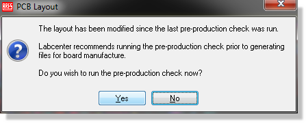
The Pre-production check (PPC) prompt
If your pre-production check reports errors we strongly recommend that you resolve them before proceeding to the manufacturing output dialogue. Please also note that pre-production check is an aid to the designer in quality assurance but not a guarantee; manual inspection of the layout is recommended and a prototype should always be made and tested before mass production.
More information on the Pre-production Check can be found in the CADCAM Output section of the online reference manual (Help Menu).
Assuming a pass you will then be provided with the manufacturing output dialogue form
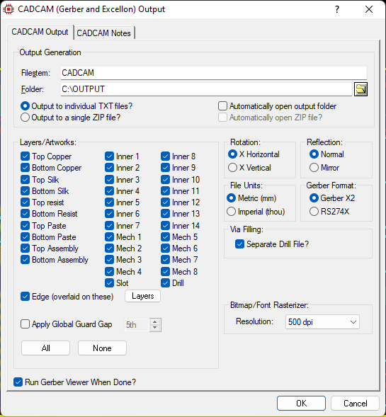
The Gerber / Excellon Output dialogue form
The options in the top section of the dialogue form are self-explanatory but there are some points of note regarding the rest of the configuration options.
The software attempts to populate the layer set with those layers used on the layout but this should always be verified. One of the most common problems with manufacture occurs when the manufacturer is not supplied with the full board information.
The Apply Global Guard Gap option will set the expansion of the resist plot around pads and vias to the distance specified when this option is checked. This will take effect on all pads and vias except those which have been manually altered on the layout. Some board manufacturers prefer to create the resist plot in house and this option could then be used to remove any resist expansion pre-manufacture. Unless otherwise directed we recommend that you leave this option unchecked.
See Also:
The Bitmap/Font Rasterizer option controls the thickness of trace used to render bitmaps and true type fonts. The higher the resolution the better tonality of the resulting bitmaps but the larger the files. It is also possible that some manufacturers have a minimum width requirement and in such cases it may be necessary to reduce the DPI settings to conform with this. Generally speaking however, the default settings are fine.
The option at the bottom left allows you to automatically load your output into either the Labcenter Gerber Viewer (CADCAM Output) or the Valor ODB++ Viewer (ODB++ Output). This is useful if you want to verify the output fileset before passing to your manufacturing house.
If you intend to panelize the board you should use the Gerber X2 output in the CADCAM Output command, then close the project, open the gerber module and import your CADCAM files, selecting Panelization Mode from the resulting dialogue form. Panelization is only available with Gerber X2 output - you cannot create panels from RS274X Gerber.
See Also:
Panelization (Reference Manual)
Finally, the Notes tab allows us to insert any relevant information or special considerations for the manufacturer. This is very important when we have specified a slotting layer as there is no standard way to pass this information through. A simple note that the information on MECH1 is for slotting will suffice, although you can choose to include your manufacturing notes from the Project Notes module (detailed next) if you prefer.
Project Notes
Proteus includes a "Project Notes" module, which can be used to record any notes about the project, provide information for PCB fabrication / assembly, and/or check details regarding aspects of the project such as whether length-matches are within the specified tolerances. A number of automated Fields and Project Data elements are available within the module, to assist with report generation and maintenance. More than one Note document can be included in a project, with certain types of notes having special purposes, such as being automatically included in CAD/CAM output or automatically appended to Bill of Materials output.
The Project Notes module is accessed via the "Project Notes" button on the toolbar.
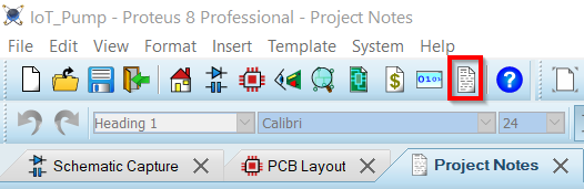
Project Notes Module
A "Generic Note" will open by default, however other types of notes (and/or additional Generic Notes") can be added from the File menu.
We will add the project name and version as a header to our report. Select the "Heading 1" style, and then select Insert -> Fields -> Title. The title is taken from the Design Properties, which we specified in the schematic (see the Bill of Materials section of the Schematic tutorial; Schematic Module -> Design menu -> Edit Design Properties). Next, insert a space and then add the project version using the "Revision" field. You may then wish to type "Project Notes" in order to complete the title. On the next line, change to the "Paragraph Style" and insert the project "Modified Date (long)" field. Note that other text, images, tables, and so on can be added to the report as you like, similar to a standard text editor; in the following screenshot, a company logo has been added at the top of the report.

Project Notes Header
Note that document templates may be saved using the Template menu, and that these will then be available to select from when creating a new Project Note.
A number of Project Data elements are available to be included in the report:
| Project Data | Description |
| Schematic Grid References | Table listing the location of each part on the schematic grid (if available, see Component Placement Report). |
| PCB Board Stackup | Table detailing the PCB layers, as specified under the Layer Stackup in the PCB Layout module. |
| PCB Layer Stack Profile | Graphical representation of the Layer Stackup. |
| PCB Image Output | PCB image; a number of options can be specified when generating the image; the Assembly Plot mode can be useful during board assembly. |
| PCB Image Output | PCB image; a number of options can be specified when generating the image; the Assembly Plot mode can be useful during board assembly. |
| PCB Drill Table | Table detailing all the drill types required during the PCB manufacturing process. |
| PCB Fiducials | Table detailing all of the PCB fiducial locations; useful during the PCB assembly process. |
| Length Matches | Report of all length-matched tracks on the PCB, including whether or not they are within the specified tolerances. |
| Differential Pairs | Report of all differential pairs on the PCB, including whether or not they are within the specified tolerances. |
| Design Rules | Report of all the design rules which are active in the project |
| Variant Comparison | Report of the different types of variants in a project, detailing which parts are fitted or have a different part number, for each variant. |
| Single Pin Nets | Report of all "Single Pin Nets" within a project, a "Single Pin Net" being where any pin or terminal is not connected to any other pin or terminal in a project (more on this to follow). |
| PCB Image Output | PCB image; a number of options can be specified when generating the image; the Assembly Plot mode can be useful during board assembly. |
Project Data elements are inserted in the same way as Field elements.
The "Single Pin Net" element warrants some additional discussion; this report can be used to help highlight cases where, for example, terminals have accidentally been misnamed and are not actually connected (such as one terminal being labelled "LED_LEVEL_HIGH" and the other terminal being labelled "LED_LEVEL_HI"). Unused/unconnected component pins will also turn up in the report, and can be excluded from it by connected the unused pins to "NC" terminals.
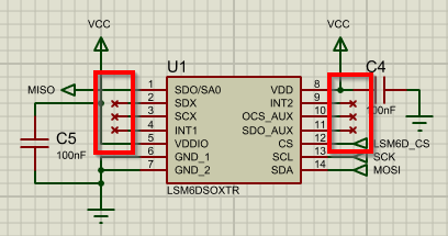
"NC" Terminals
Add some Project Data elements, such as a Fiducial Report (PCB Fiducials) and Assembly Plot (PCB Image Output), to your report, in order to get a feel for them.
Project Data elements in a report are not automatically updated, and refresh of these can be done using the "Reload Project Report" command on the Edit menu, or by right-clicking on a Project Data element and selecting "Reload Project Data".
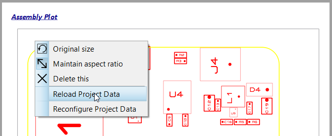
Refreshing a Project Data element
The exact details of what to include in the report (if any) will depend on your internal business processes, and the information required by your PCB manufacturer / assembler. For an example Project Notes report, please open the "IoT Pump (Complete)" sample design.
See Also:
Reference Manual - Manufacturing Report
Project Notes : PCB Specification Notes.
Having configured all the necessary options, we can generate the files and send for manufacture - bringing us to the end of this tutorial!