FREQUENCY ANALYSIS
Overview
With Frequency Analysis you can see how the circuit behaves at different frequencies. Only one frequency is considered at a time, so the plots are not like those seen on a spectrum analyser, where all frequencies are considered together. Instead, the simulation is similar in effect to connecting a frequency generator to the input, and looking at the output with an AC voltmeter. As well as the magnitude, however, the phase of the probed signal can also be seen.
Frequency analysis produces frequency response or Bode plots. It is useful in checking that filters are behaving as expected, or that amplifier stages will work correctly across the required frequency range.
Frequency graphs can also be used to plot small signal input and output impedance against frequency.
Method of computation
Frequency analysis is performed by first finding the operating point of the circuit, and then replacing all the active components with linear models. The internal capacitances of the active devices are calculated at the operating point, and assumed not to vary much over the working voltage swings of the circuit. All the generators, apart from frequency reference generators (see below) are replaced by their internal resistances. This causes power lines to be effectively connected together, as is normally the case during frequency computations.
The analysis is then performed with complex numbers in a linear fashion. The frequency of interest is stepped from the start frequency to the stop frequency, and the linear nature of this analysis makes it typically much faster than transient analysis, even though complex numbers are used.
It is important to remember that frequency analysis assumes a linear circuit. This means that a pure sine wave at the input will produce a pure sine wave at the output, over all the frequencies probed. Of course, no real active circuit is purely linear but many are close enough to allow this form of analysis. There are also circuits which are not at all linear, such as line repeaters with schmitt trigger inputs. For non-linear circuits the term 'frequency response' has no real mathematical meaning, and so any frequency simulation will not produce meaningful results. Should you be interested in the frequency domain behaviour of such circuits, then Fourier analysis is much more appropriate.
Using Frequency Graphs
To calculate the magnitude of sine waves at the output, we must inject a reference sine wave at the input. PROSPICE will do this automatically, but needs to know where the input of the circuit is. To do this, you must give each frequency graph a reference generator to tell the simulator where to inject the reference signal. There are three ways of doing this:
- Use the Reference
field on the Edit Frequency Graph dialogue form to select an input
generator. This object can be any ordinary single pinned generator
object, or the FREQREF primitive from the ASIMMDLS library.
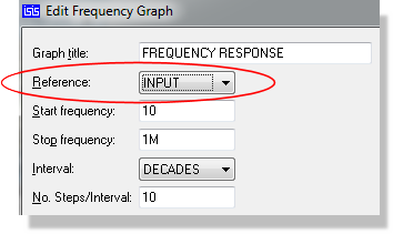
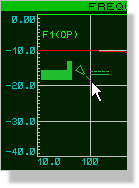
- Tag and drag any analogue generator onto the
frequency graph.
- Use the Add Phasor Trace dialogue form and select
Reference as the axis.
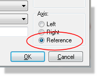
The FREQREF primitive is useful for defining models that drive the circuit, a microphone model for example. This could contain an explicit named generator, used as a reference when the effects of the rest of the microphone model (such as modelled frequency response) need to be taken into consideration.
The second and third techniques will be used more often. The action of dragging a generator onto a frequency graph is different to dragging it onto a transient graph. Instead of adding the generator's probe, the generator becomes the circuit reference point, and a message confirming the choice is written to the simulation log. The generator need not be a Sine generator: DC, Pulse and Pwlin will all work as well. A digital generator cannot be used as a reference and will be refused. If you want to add the generator as a probe, it can still be done using the Add Phasor Trace dialogue form.
The magnitude of the reference is always 1 volt and the phase is always 0 degrees; neither is adjustable. The internal resistance of the reference generator will follow whatever was defined for the generator in the first place. The 1 volt magnitude is what the dB calculations are referred to, so 0dB is 1 volt. Very small values are limited to -200dB to avoid taking the logarithm of zero.
The Frequency Axis
The range of the sweep and the way it is divided up are set on the Edit Frequency Graph dialogue form. Start frequency and Stop frequency give the extremes, and default to 10Hz and 1MHz. Interval chooses how the range is divided, offering DECADES, OCTAVES or LINEAR, and No. Steps/Interval sets how many points are computed within each interval. With the defaults of DECADES and 10 steps, a sweep from 10Hz to 1MHz computes 10 points per decade. Simulation time is roughly proportional to the total number of points, so raise the step count only where the extra resolution is needed.
The x-axis is normally drawn on a logarithmic scale, which suits the decade and octave interval settings. It switches to a linear scale when the Interval is set to LINEAR, and also when the span currently displayed is narrow enough that a logarithmic scale would serve no purpose, which happens when you zoom in closely.
The Y-Axes
Frequency graphs always have both left and right y-axes. The left y-axis is used to display the magnitude of the probed signal, and the right y-axis is used to display the phase. If you drag a probe onto the left of the graph, it will display magnitude; if you drag it onto the right, the phase. The left y-axis may be displayed either in dBs or normal units, controlled by the Y Scale in dBs option, and the right y-axis is always in degrees.
See Manual Y-Axis Configuration for information on defining y-axis limits.
To see the frequency response of a circuit:
- Place probes around the circuit at points of interest.
- Place a Frequency graph.
- Add the probes to it. Add to the left for magnitude, and to the right for phase. You may well want to add probes twice in order to see both phase and magnitude.
- Edit the graph by pointing at it and selecting Edit Graph... from the Graph menu, then set the required start and stop frequencies, the interval and step count, and any Simulation Control Properties required.
- Press the space bar to invoke PROSPICE.
The sample designs Zin.pdsprj and Zout.pdsprj, in the Graph Based Simulation samples folder, show how to combine frequency graphs with trace expressions to plot input and output impedance.
See Also: