THE DIGITAL SIMULATION PARADIGM
The DSIM State Model
You might think that a digital simulator would model just high and low states, but DSIM models rather more than that. A DSIM state carries two pieces of information: its polarity, which is high, low, undefined or floating, and its strength, which is a measure of the amount of current the output can source or sink. Strength becomes relevant when two or more outputs are connected to the same net, because the stronger one wins.
Crossing the four strengths that drive a net with the three polarities they can drive gives the following set of states:
| Strength | Logic 1 | Logic 0 | Undefined | Typical source |
Power |
PHI |
PLO |
PUD |
A power rail. |
Inject |
IHI |
ILO |
|
A signal injected by a generator. |
Strong |
SHI |
SLO |
SUD |
An active output. |
Weak |
WHI |
WLO |
WUD |
A passive output such as a pull-up resistor, or a mid voltage arriving from an analogue source. |
One further state completes the set. FLT is the floating state, the high impedance condition of an inactive output, and it has neither a driving strength nor a defined polarity.
For example, if an open-collector output is wired through a resistor to VCC, then when the output is pulling low, both a Weak High and a Strong Low are applied to the net. The Strong Low wins, and the net goes low.
This scheme permits DSIM to simulate circuits with open-collector or open-emitter outputs and pull up resistors, and also circuits in which tristate outputs oppose each other through resistors. However, it is important to remember that DSIM is a digital simulator only and cannot model behaviour which becomes decidedly analogue. For example, connecting overly large resistors up to TTL inputs would work in DSIM but would fail in practice due to insufficient current being drawn from the inputs.
Contention
If two tristate outputs both go active onto a net and drive in opposite directions, the result is a contention. Contention is not a thirteenth state: it is a flag raised on whichever state the net resolves to, and two consequences of that follow which are not obvious.
- A contended net keeps its strength. Two equal strength drivers pulling against each other produce a contention at that strength, and a third, stronger driver on the same net will still override it. Neither output winning is therefore only true against an equal strength opponent.
- Inject strength never raises contention. A generator driving against a model output simply wins, with no contention flagged and no warning, which is what you want when you are injecting a test signal into a working circuit but surprises people who expect the clash to be reported.
On a digital graph trace and in the status line, the twelve states are collapsed into six display keywords, and a contended net is shown there as CON.
See Also:
The Undefined State
Where an input to a digital model is undefined, this is propagated through the model according to what might be described as common sense rules. For example, if an AND gate has an input low, then the output will be low, but if all but one input is high, and that input is undefined then the output will be undefined.
- Edge triggered devices require a transition from a positively defined logic 0 to logic 1 (or vice versa) for an edge to be detected. Transitions from 0 or 1 to undefined and back are not counted as edges.
- The more complex sequential logic devices (counters, latches and so on) will often resolve undefined inputs to a logic 0 or logic 1, according to the coding of their internal logic. This is not unlike real life.
Floating Input Behaviour
It is common, if not altogether sound practice, to rely on the fact that unconnected TTL inputs behave as though connected to a logic 1. This situation can arise both as a result of omitted wiring, and also if an input is connected to an inactive tristate output. DSIM has to do something in these situations since the internal models assume true logical behaviour with inputs expected to be either high or low.
This is catered for through the FLOAT property. This may be assigned either directly to a component, or to an Interface Model. In particular, the interface model for TTL parts has the assignment:
FLOAT=HIGH
which causes floating inputs to be interpreted as logic 1 levels.
To specify that floating inputs be taken as logic 0, use
FLOAT=LOW
Otherwise, floating inputs will be taken to be at the Undefined state.
The interface models that carry FLOAT=HIGH are TTL, TTLLS, TTLS, PLD, 8051, AT89 and RS232. The high speed CMOS families, 4000 series CMOS and every processor family other than the two named above do not, so their floating inputs go to Undefined rather than to logic 1. This is a real behavioural difference between families and it catches people who assume TTL behaviour is universal.
See Also:
Mixed Mode Interface Models (ITFMOD)
Glitch Handling
How a digital simulator should handle models subjected to very short pulses is a genuinely difficult question. The fundamental problem is that, under these conditions, a major assumption of the DSIM paradigm, that the models behave purely digitally, starts to break down. For example, a real 7400 subjected to a 5ns input pulse will generate some sort of pulse on its output, but not one that meets the logic level specifications for TTL. Whether such an output pulse would clock a following counter is then a matter dependent on very much analogue phenomena.
The best one can do is to consider the extremes, namely:
- A 1ns input pulse will not propagate at all.
- A 20ns pulse will come through nicely.
Somewhere in between, the gate will cease to propagate pulses properly and could be said to suppress glitches. This gives us the concept of a Glitch Threshold Time, which can be an additional property of the model along with the usual TDLH and TDHL.
Another subtlety concerns whether the glitch is suppressed at the input or the output of a model. To resolve this, consider a 4-16 decoder driven from a ripple counter as shown below.
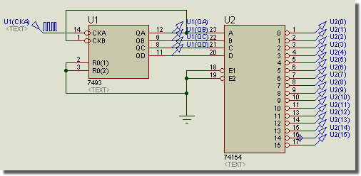
4-16 Decoder driven from a Ripple counter
The outputs of the ripple counter are staggered, and thus the possibility arises of the decoder generating spurious pulses as the inputs pass through intermediate states. This situation is shown in the following graph:
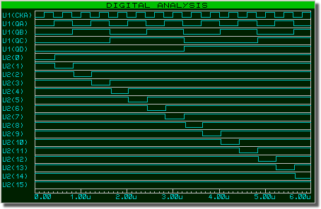
Digital Graph analysis of the decoder
Taking the first glitch as an example of the phenomenon, as U1(QA) falls for the first time, it beats the rise of U1(QB) and an intermediate input state of 0 is passed to the decoder for approximately 10ns. The question is whether the decoder can actually respond to this or not, and even more to the point, what would happen if the input stagger was only 1ns or 1ps? Clearly, in the last two cases the real device would not respond, and this tells us that we must handle glitches on the outputs rather than the inputs. This is because, in the above example, the input pulses are all relatively long and would not be considered glitches by any sensible criteria.
The really interesting part of this tale is that, if you build the above circuit, it will probably not glitch. It is very bad design certainly, but the TDLH and TDHL of the 154 are around 22ns and this makes it a tall order for it to respond to a 10ns input condition. With the individual components we tried, no output pulses, other than perhaps the slightest twitches off the supply rails, were measurable.
To provide control over glitch handling, all the DSIM primitives offer user definable Glitch Threshold Time properties named TGxx, where xx is the name of the relevant output. Our TTL models are defined such that these properties can be overridden on the TTL components, and the values are then defaulted such that the Glitch Threshold Times are the average of the main low-high and high-low propagation delays. Setting the Glitch Threshold Times to zero will allow all glitches through, should you prefer this behaviour. The graph, above, was created by attaching the property assignment TGQ=0 to the 74154.
The glitch and delay properties are ordinary component properties. Point at the part, press CTRL+E, and add the assignment in the Edit Component dialogue form like any other property.
Finally, it is important to point out that if the Glitch Threshold Time is greater than either of the low-high or high-low propagation delays, then the Glitch Threshold Time will be ignored. This is because, after an input edge, and once the relevant time delay has elapsed, the gate output must change its output: it cannot look into the future and see whether another input event that might cancel the output is coming. Consider a symmetric gate with a propagation delay of 10ns and a Glitch Threshold Time of 20ns. At t=0ns the input goes high and at t=15ns the input goes low. You might expect this to propagate, with the output going high at t=10ns and low again at t=25ns, so producing a pulse of width 15ns which would be suppressed, since it is less than the Glitch Threshold Time. The reason the pulse is not suppressed is that, at t=10ns, the output has to go high. It cannot remain low for a further 20ns on the off chance that a second edge comes along, as in our example, producing an output pulse it would then need to suppress. Once the output has gone high at t=10ns then the second edge (at t=25ns) is free to reset it.