DIGITAL TRANSIENT ANALYSIS
Overview
Digital graphs display what you would normally expect to see on a logic analyser. The x-axis shows the advance of time whilst the y-axis shows a vertical stack of signals. These can be either single data bits, or a representation of the binary values carried by a bus.
Method of Computation
Digital transient analysis is computed using a technique known as Event Driven Simulation. This is different from analogue transient analysis in that processing only occurs when some element of the circuit changes state. In addition, only discrete logic levels are considered and this enables component functionality to be represented at a far higher level. For example, we can think of a counter in terms of a register value that increments by one each time it is clocked, rather than in terms of several hundred transistors. This makes event driven simulation several orders of magnitude faster than analogue simulation of the same circuit.
The Boot Pass
The purpose of the boot pass is to define the initial states of all nets in the circuit, prior to the simulation proper. The boot pass is carried out as follows:
- All input pins connected to the VCC and/or VDD nets are deemed to be high.
- All input pins connected to the GND and/or VSS nets are deemed to be low.
- All input pins connected to a net to which a generator is connected are deemed to be at the same state as the INIT property of the generator.
- All remaining pins are deemed to be initially floating.
- All models are requested (in no set order) to evaluate their inputs and set their output pins accordingly. As each output pin is set, the state of the net to which the pin connects is re-evaluated.
- As nets change state, models connected to them are asked to re-evaluate their outputs. This process continues until a steady state is found.
The Event Processing Loop
Following the boot pass, DSIM begins the simulation process proper. The simulation is carried out in a loop which passes repeatedly through the following two steps:
- All the state change events for the current time are read off a queue and applied to the relevant nets. This process results in a new set of net states.
- Where a net changes state, all the models with input pins attached to the net are re-simulated. Where their outputs change state, this creates new events which are placed on the event queue.
Of course, different models will create events which fall due for processing at different times. The DSIM kernel thus has to order all the new events created at the end of each cycle round the loop.
It is also worth pointing out that our scheme quite happily supports models which have a zero time delay. In this context, events generated with the same time-code are processed in batches (one batch equals one trip round the loop), according to how they were generated.
Termination Conditions
Simulation stops when one of the following occurs:
- The specified stop time is reached.
- The event queue becomes empty. This means that the circuit has reached a permanently stable condition.
- The run is suspended, either by a breakpoint or a watchpoint in a processor model, or because the kernel has processed as many events as it is allowed to in a single pass and is yielding control back to the application.
- An error is logged. The most common error of this kind is a logic race condition, described below.
Logic Race Conditions
A logic paradox with zero time delay can leave the current time unable to advance, however many times the kernel goes round the event processing loop. DSIM detects this by counting the batches of events processed at a single time point. Once the count is exhausted the simulation stops and the message Logic race condition detected during transient analysis. is written to the simulation log. The same situation during the operating point analysis is reported as a warning rather than an error.
The limits are netlist properties, so a design that genuinely needs more settling can raise them. MAXRACEEVTS sets the number of batches allowed at one time point and defaults to 32; MAXBOOTEVTS applies during the boot pass and defaults to 128; MAXRUNEVTS sets the number of events processed before the kernel yields and defaults to 1000000.
A race condition usually means something is unstable about the design, perhaps a very high frequency oscillation, or a feedback path built entirely from models with no propagation delay.
Using Digital Graphs
To perform a transient analysis of a digital circuit:
- Add generators as necessary around the circuit, to drive the circuit inputs.
- Place probes around the circuit at points of interest. These may be at points within the circuit, as well as obvious outputs.
- Place a Digital graph.
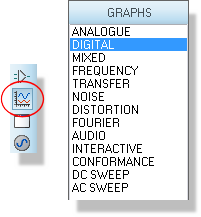
A digital graph placed on the schematic
- Add the probes (and generators, if desired) to the graph.
- Edit the graph and set up the simulation stop time required, as well as labelling the graph and setting control properties if required.
- Invoke the Simulate Graph command against the graph, or press the space bar.
Only digital generators should be used to generate digital signals. Note in particular that the Pulse generator is intended for generating analogue pulses. The digital equivalent is the Single Pulse sub-type of the digital generator. See Digital Generators.
Only voltage probes should be used for probing digital nets. Using current probes will force PROSPICE to perform a mixed mode simulation.
See The Simulation Process for general information on how to simulate a graph.
See Placing Generators for information on placing generators and Placing Probes for information on placing probes.
See Adding Traces To A Graph for more information about adding probes to graphs.
How Digital Data is Displayed
Normal Traces
The graph readout describes the state of a single bit trace with one of six keywords. These are a summary of what the simulator engine is actually modelling: DSIM works with a larger set of drive states, and the readout groups them by level and strength so that the display stays legible.
| STATE TYPE | KEYWORD | GRAPHICAL APPEARANCE |
| Strong High | SHI |
High level, in the digital trace colour |
| Weak High | WHI |
High level, in the digital trace colour |
| Floating | FLT |
Mid level, in the float colour |
| Contention | CON |
Mid level, in the float colour |
| Weak Low | WLO |
Low level, in the digital trace colour |
| Strong Low | SLO |
Low level, in the digital trace colour |
The waveform is drawn in a single colour for every state that has a defined level, so a high is distinguished from a low by the position of the trace and not by its colour. Only the mid level states are drawn differently, and both of them use the float colour. Both colours are set in the Graph Colour Configuration form, reached through Set Graph & Trace Colours; the defaults are cyan for the digital trace and white for a floating signal.
You can therefore determine the state of a trace at a particular time either by looking at the position of the trace line, or by opening the graph window, positioning a cursor over the desired position, and reading the state off the status line. The logic levels at the cursor position are also displayed just to the right of the trace labels.
Contention is easier to spot on the schematic than on a graph. During an interactive simulation with Show Logic State of Pins? enabled, the pin state squares show contention in yellow, alongside red for a high, blue for a low and grey for a floating or undefined pin. On a digital graph trace contention is drawn in the float colour and cannot be told apart from a floating signal by colour alone.
See The Digital Simulation Paradigm for the state model the simulator engine works with.
See Taking Measurements for pin state display during interactive simulation.
Bus Traces
Bus traces (resulting from the placement of voltage probes on bus wires) display the hex values of the bus bits between cross over lines:

Bus Traces
Where one or more of the bus bits is neither high nor low, the bus line is drawn at the mid level. Also, if the edge transitions are too close together to display the hex value, then it is omitted. The value can still be established by positioning a cursor over it.
See Also: