ANALOGUE TRANSIENT ANALYSIS
Overview
This graph type represents what you might expect to see on an oscilloscope. The x-axis shows the advance of time, whilst the y-axis displays voltage or current. We often refer to this type of analysis as Transient Analysis because it takes place in the time domain.
Transient analysis is perhaps the most commonly used form of analysis. Everything that you would measure with an oscilloscope on a real prototype can be measured on an analogue graph. It can be used to check that the circuit operates in the expected manner, to take quick measurements of gain, to assess visually the way in which a signal is distorted, to measure the current flowing from the supply or through individual components, and so on.
Method of computation
Technically speaking, this type of simulation can be referred to as Non-Linear Nodal Analysis, and is the form of computation used by all SPICE simulators. Considering a single point in time, every component in the circuit is represented as a combination of current sources and/or resistors. This arrangement can then be described as a set of simultaneous equations using Ohm's law and Kirchoff's laws, and the equations solved by Gaussian Elimination. Each time the equations are solved, the values of the current sources and resistors are adjusted by laws built into the component models and the process is repeated until a stable set of values results.
For a simulation involving the advance of time there are two separate stages. The first task is to compute the operating point of the circuit, that is the voltages around the circuit at the very start of the simulation. This is then followed by considering the effect of advancing time on the circuit, and re-calculating the voltages at every step, iterating to convergence as described above. The size of each time increment is crucial to the stability of the calculations, and so PROSPICE will adjust it automatically within user defined limits. Circuits that are changing quickly, such as high switching speed line drivers, need smaller time steps and so require more effort to simulate than circuits that change more smoothly. The use of time step control and iterative solutions all adds up to a great deal of calculation, which can make transient analysis seem comparatively slow.
Since the algorithm involves iteration, there is always a possibility that the solution will not converge. Most commonly this happens at the initial time-point, meaning that the simulator cannot establish a stable or unique set of values for the operating point. Occasionally, however, it can occur further into a simulation where the circuit behaviour at a particular time becomes highly unpredictable. PROSPICE implements a number of techniques to help avoid such problems, but it is not impossible to defeat. This said, being based on Berkeley SPICE3F5 it is as good as you are going to get.
Using Analogue Graphs
Analogue graphs may have either just the left y-axis, or both left and right y-axes. Probes can be placed on a particular axis in two ways.
By tagging and dragging the probe to the appropriate side of the graph:
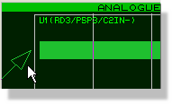
Adding a Probe on to the graph
By using the Add Transient Trace dialogue form:
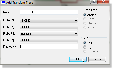
Adding Traces to a graph via the Graph menu
See Adding Traces To A Graph for more information about adding traces to graphs.
It is often convenient to use the left and right y-axes to separate traces with different units. For example, if both voltage and current probes are displayed, then the left side can be used for voltage and the right side for current.
An analogue graph will not accept a digital trace. On the Add Transient Trace form the Digital trace type is greyed out, and dragging a digital probe on to the graph has no effect. If you tag a digital probe and use the quick add route, the probe is added as an analogue trace instead, which plots the interface voltage rather than the logic state and is rarely what you want. To display logic levels alongside waveforms, use a Mixed graph.
To perform a transient analysis of an analogue circuit
- Add generators as necessary around the circuit, to drive the circuit inputs.
- Place probes around the circuit at points of interest. These may be at points within the circuit, as well as obvious outputs.
- Place an Analogue Graph.
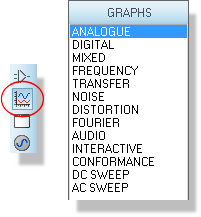
- Add the probes (and generators, if desired) to the graph.
- Edit the graph by pointing at it and selecting
Edit Graph... from the Graph
menu. Set up the simulation stop time required, as well as labelling
the graph and setting control properties if required.
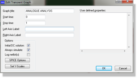
- Start the simulation by either selecting the Simulate Graph command or pressing the space bar.
The graph fills in as the run proceeds, so you can watch the response take shape and stop early if it is clearly wrong. This is controlled by the Live Updates option on the edit dialogue form, which is enabled for new graphs.
See Live Updates for more information.
See Manual Y-Axis Configuration for information on defining y-axis limits.
See Placing Generators for information on placing generators, and Generators for a discussion of the different types of analogue generator.
Defining Analogue Trace Expressions
You will normally want to add voltage and current probes to your graphs, to see the operation of a circuit. However, in an analogue transient analysis it is possible to create traces that are mathematical expressions based on probe values. For example, suppose a circuit output has both a voltage and current probe placed on it. By multiplying these values together, the output power at this point will be plotted.
To plot the output power:
- Add a current probe and a voltage probe to the circuit output.
- Invoke the Add Transient Trace dialogue form for the graph, using Add Traces... on the Graph menu or CTRL+T.
- Assign the voltage probe to P1.
- Assign the current probe to P2.
- Alter the expression to read P1*P2.
- Click on the OK button.
- Press the space bar to invoke the simulation.
See Also: