THE SIMULATION PROCESS
Demand Driven Simulation
When we designed Proteus, one of our major goals was to make the use of simulation software much more intuitive than it has previously been. Much of the problem with previous simulation packages stems from the fact that number crunching parts were written first and other aspects such as displaying the results graphically were added on later, almost as an afterthought. This tends to result in a fragmented way of working in which you run one program to draw the schematic, another to actually simulate the circuit, and yet another to display the results.
Proteus is very different in that, having drawn the circuit, you start by answering the question of what you want to see by means of placing and setting up a graph. This graph then persists until you delete it, and each time you want to see the effect of a change to the circuit, you just update the graph by pointing at it and pressing the space-bar. We call this Demand Driven Simulation since Proteus must work out from the graph what actually requires simulating, rather than you having to do it textually. Furthermore, you can place several graphs which perform different experiments with each one 'remembering' a different setup for the simulators.
The most important benefit of all comes from the fact that a given graph defines a set of points of interest in the design by virtue of the probes that have been assigned to its traces. Proteus is then able to use this information to figure out which parts of the design actually need to be simulated, rather than you having to carve the design up manually. It follows that a complete design, ready for PCB layout, can be simulated without massive editing, even if you only want to simulate particular parts of it.
A further benefit arises from the fact that there is no risk of forgetting to undo modifications made for simulation purposes. There are none to undo, because the probe and generator objects that you do place are ignored when generating netlists for PCB layout.
Executing Simulations
Once a graph has been placed with probes and generators assigned to it, you can initiate a simulation by pointing at the graph and pressing the space-bar. Proteus then determines which parts of the design need to be simulated in order to update the graph, runs the simulations, and displays the new data.
Throughout the simulation process, a simulation log is maintained. In general, the log contains little of interest. However, you will need to view the log at the end of the simulation run if simulation errors have occurred, or if you have asked for the simulation netlist to be logged by selecting Log netlist(s): on the graph's edit dialogue form, or if the analysis type results in data that is not amenable to graphical display, as an analogue Noise analysis does.
To update a graph and view the simulation log:
- Either ensure the graph you want to update is the current graph and then select the Simulate Graph command, or place the mouse pointer over the graph you wish to update and press the space bar.
- If the simulation aborted part way through, you are asked Load partial results?. Answering Yes loads the data captured up to the abort and displays it on the graph; answering No opens the simulation log instead. A fatal error produces a different prompt, which offers only to show the log.
Whether or not errors occurred, you can view the simulation log at any time by right clicking on the graph and selecting the View Simulation Log command, or by pointing at the graph and pressing CTRL+V.
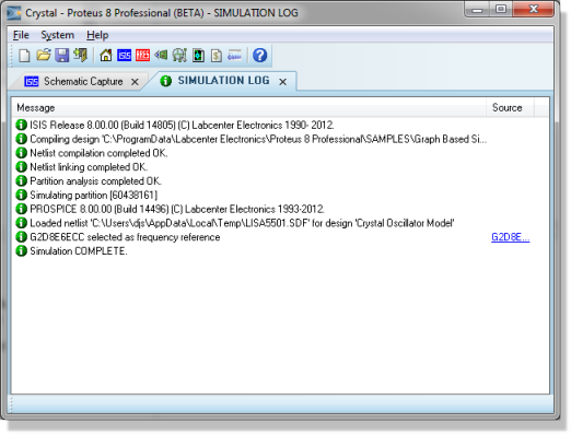
The simulation log for a graph
Proteus can also interpret a simulated graph for you, taking numeric measurements from the traces and commenting on the response. See Placing Graphs and Running Simulations in the EDAi manual.
Live Updates
A transient graph fills in as the simulation runs, rather than waiting for the run to finish. The traces extend across the graph a few times a second while the simulator works, so you can see the response taking shape and stop a run early if it is clearly not doing what you expected. Proteus limits itself to around twenty of these updates a second, so the display keeps up with a fast run without the drawing becoming the bottleneck.
Live tracing is controlled by the Live Updates option in the Options group of the graph's edit dialogue form. New graphs have it enabled, with the exception of conformance graphs, where it is off by default. The setting is stored with the graph, so it travels with the design.
Only the transient family of graphs can update as they run: analogue, digital and mixed transient graphs, along with audio, interactive and conformance graphs. Frequency, DC sweep, AC sweep, transfer, noise, distortion and Fourier graphs produce their results only at the end of the run and are unaffected by this option.
Drawing the traces repeatedly does cost a little time. If a long run feels sluggish, clearing Live Updates for that graph is worth trying, along with the other measures described in How to Make Simulations Run Faster.
What Happens When You Press the Space-Bar
When you update a graph, either using the Simulate Graph command on the Graph menu or its space-bar keyboard short-cut, a great deal of analysis and processing occurs over and above the actual analogue or digital analyses themselves. We now outline in brief the various steps in this process:
- Netlist compilation - this is the usual process of tracing wires from pin to pin, and producing a list of components and a list of pin to pin connection groups, or nets. The resulting netlist is held in memory at this stage.
- Netlist linking - some components are modelled
using sub-netlists or model files
which are generally kept in one of the folders named by the
User Simulation Model and Module Folders
setting, on the Simulator Settings
tab of the System Settings
dialogue (System menu). Many models are supplied with Proteus and
you can, of course, create your own as well. You can think of a model
as being a child sheet of a hierarchical design in which the parent
object is the component to be modelled.
Each time a component modelled in this way is encountered, the original part is removed from the netlist and replaced by the contents of the model file, with the inputs and outputs of the model connected in where the original component's pins were.
At the end of this process, every component left in the netlist should have a PRIMITIVE property, which means that it can be directly simulated by PROSPICE. - Partitioning - Proteus then looks at the points
where you have placed probes and traces back from these to where
you have injected signals. A signal is deemed to be injected by any
of: a power rail, a generator with its Isolate
Before flag set or tape output. This analysis results in the
establishment of one or more partitions that may need to be simulated.
Further analysis then works out the order in which they must be simulated. For example, if partition A has an output that connects to an input of partition B then clearly A must be simulated first. If it turns out that B has an output driving A as well, then all is lost: it is up to you to use tape objects in such a way that cyclic dependencies do not occur.
Yet more analysis then establishes whether there are any existing results in the folder named by the Path to folder for simulation results setting, on the Simulator Settings tab of the System Settings dialogue (System menu), that relate to identical simulation runs for any of the current set of partitions. If there are, and if the partition concerned is not driven by a partition which is itself being re-simulated, then Proteus does not bother re-simulating the partition, but uses the existing results instead. It follows that if you are working on the back end of a design, there is no need to keep re-simulating the front end.
This optimisation applies only when a graph's Always simulate: option is cleared. New graphs have it set, so by default every partition is re-simulated on each run. Stored partition results are also aged out once they exceed the disk space limit set by the Limit maximum disk space used for simulation results to: setting on the same tab, which is a second reason a partition may be re-simulated when you expected it to be reused. - Simulator Invocation - Proteus now invokes PROSPICE on
each partition in turn to carry out the actual simulation.
Each simulator invocation results in a new partition file, and progress information is also added to the simulation log which is maintained throughout the entire simulation process.
- Results Processing - Finally, Proteus accesses the partition files to build up the various traces on the graph. The graph is then re-displayed and can be opened in its own window for measurement taking and so forth.
If errors occur during any of these stages then the details are written to the simulation log. Some errors are fatal, and others are just warnings. In the case of fatal errors, the simulation log is displayed for immediate viewing. If only warnings have occurred then the graph is re-displayed and you are offered the choice of viewing the simulation log if you want to. Most errors relate either to badly drawn circuits (which cannot, for one reason or another, be mathematically solved), or to the omission or incorrect linking of model files.
See Also: