Introduction to Peltier Devices
Peltier devices are thermoelectric modules that deliver solid state heat-pumping for both cooling and heating. They also can be used to generate DC power, albeit with reduced efficiency.
Modern Peltier technology comes from the discoveries of 19th century scientists Thomas Seebeck and Jean Peltier. Seeback found that if a temperature gradient is placed across two junctions of two dissimilar conductors, an electrical current will flow through. On the other hand, Peltier, discovered the opposite effect, that a current flowing through two dissimilar conductors caused heat to be either emitted or absorbed at the junction of the materials.
How modern Peltier modules are made
A typical Peltier module consists of an array of Bismuth Telluride semiconductor pellets doped to create individual elements having N and P characteristics. The Bismuth Telluride alloy (Bi2 Te3) features better performance for the temperature range -100°C up to 200°C and so is preferred to other semiconductor alloys.
The pairs of P/N pellets are configured so that their junctions are connected electrically in series but thermally in parallel. A couple of metalized ceramic substrates provide the platform for the pellet junction and the conductive tabs that connect them all.
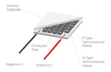 Modern Peltier Module.
Basic Peltier Theory
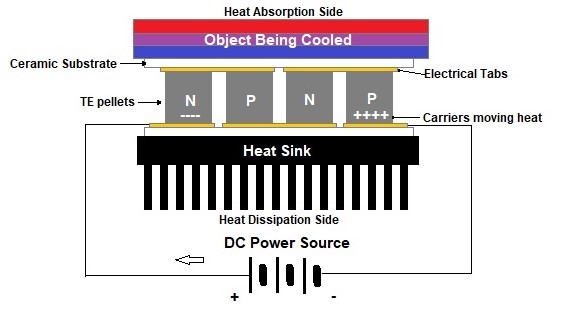
A DC voltage is provided to the module. The positive (holes in the P doped pellets) and negative (electrons in the N doped pellets) charge carriers absorb heat energy from one substrate and release heat from the opposite substrate side. The side where the heat is absorbed becomes cold and, conversely, the one side where the heat is released becomes hot. Reversing the polarity will result in reversed hot/cold sides. Heat flux (the heat pumped through the Peltier module) is proportional to the magnitude of the DC electric current.
It should be noted that Joule’s effect due to self heating of the electrical current flowing into the conductors and the Peltier module itself will act in opposition to the Peltier effect. This causes a reduction of both the available cooling and the efficiency of the device.
Also, the heat emitted to the hot side must be properly dissipated by a suitable heat sink in free or forced convection air. The following is a schematic diagram of a typical Peltier cooler.
 Peltier Cooler Example.
Benefits of Peltier Modules
The use of Peltier modules provide a number of advantages against cooling or heating conventional systems. The more obvious are:
- No moving parts - entirely solid-state, so the system can operate in any orientation and in zero gravity.
- Cooling and Heating with the same module.
- Lifetime typically over a hundred thousand hours.
- Environmentally friendly. No chlorofluorocarbons used that are harmful to the environment.
- Spot cooling. Programmatic control makes it possible to cool just a specific area only.
This makes Peltier modules useful in the most demanding industries such as medical, laboratory, aerospace, semiconductor, telecom industrial. Nevertheless, compared to conventional cooling/heating systems the efficiency of Peltier modules is limited.
Efficiency of Peltier Modules
In general, efficiency relates to the ratio of the amount of the physical work we can get out of a generic machine and the amount of the power input spent to do that work. For Peltier modules we prefer to use the term “coefficient of performance” or COP. The COP is specifically the amount of heat pumped divided by the amount of supplied electrical power.
COP = Qc / Pwatt
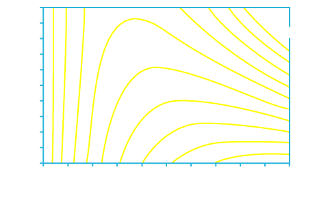
The COP depends on the heat load, input power and the required temperature differential DT across cool and hot sides. The picture below shows a normalized graph of the COP vs. I/Imax (the ratio of input current to the module’s Imax specified into the datasheet). Each line corresponds to a constant DT/DTmax (the ratio of the required temperature differential to the module’s DTmax specs.
 COP Curves for Peltier Module.
This curve refers to a single Peltier stage application. The best COP is typically limited to 0.3 to 0.7 for either cooling and heating application. When cooling with Peltier elements there are some golden rules:
- I/Imax when DT < 25°C should be from 0 to 0.33 Imax.
- I/Imax when DT > 25°C should be in the middle of 0.33 – 0.66 Imax.
- Try hard to cool the hot side as much as possible while cooling (heat sink, fan).
Ways to Improve Peltier Efficiency
There are three common rules for improving the Peltier efficiency.
- Reducing DT by optimising heat sink. Forced convection will help.
- Minimize heat losses by isolating the cooled area or the most of.
- Optimize COP by selecting the proper Peltier module of adequate power. The COP may also be optimized by using multiple Peltier modules.
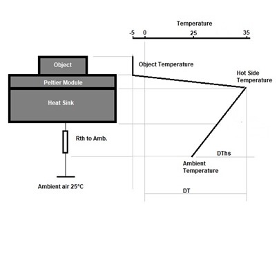
The suited heat sink must provide the correct thermal resistance to ambient (Rth) in order to reduce the hot temperature side. Of course smaller the Rth the bigger the heat sink. Using forced air convection by a fan might be a suitable solution for getting a small Rth with reasonably sized heat sink. The simplified schematic below represents a generic cooling application. The object is cooled down to -5°C by the cool side of Peltier module. The hot side of Peltier is at 40°C without heat sink, that is DT=45°C. The heat sink dissipates the heat to ambient which is at 25°C. With the proper heat sink Rth value and considering the ambient temperature at 25°C, the heat sink can dissipate 10°C and so the new DT is 40°C.
 Peltier Heat Sink.
Where possible is often beneficial to thermally insulate the object to be cooled and all other cooled surfaces. This means ambient temperature has less effect over the Peltier and it both reduces the total power dissipation and optimizes the COP. The insulation material is often polystyrene or other insulation material. In modern aerospace application silica aerogels can be used.
The Proteus Peltier Model
Proteus version 8.15 includes a realistic simulation model for generic Peltier modules. The most relevant parameters incorporated in the Proteus model of the Peltier module include the Seebeck Coefficient (SM), the Electrical Resistance (RM) and the Thermal Conductance within a large range of temperatures from -100°C to +150°C.
These parameters are provided in real-time to the SM, RM, and KM pins which are available on the Peltier device part in the Proteus Transducers library. These pins do not exist in the real hardware Peltier modules; they are only made available to the user on the schematic for diagnostic purposes. We will see a possible use of the RM simulated value to confirm the output voltage of Peltier module as power generator for a calorimeter application.
 Schematic Part in Proteus.
Finally, the QC and QH library part pins are not electrical but thermal connections. We will see their use in the example provided underneath.
What the Proteus Peltier Model Simulates
Proteus allows the simulation of most of thermoelectric module performances, including:
- Input current through the module expressed in Amperes, if powered in constant voltage.
- Input voltage to the module expressed in Volts, if powered in constant current.
- Hot side temperature (Th) of module expressed in Celsius.
- Cold side temperature (Tc) of module expressed in Celsius.
- Cold side heat (Qc) of module expressed in Watts.
- Hot side heat (Qh) of module expressed in Watts.
- Joule effect due to self heating caused from the input current through the module.
These allow the simulation in both heating and cooling mode and can be used to predict the module(s) performance and estimating the whole thermal system based to Peltier module.
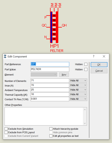 Parameter Setting in Proteus.
The most relevant parameters are:
- Number of Elements
- Imax (A)
These two parameters define the power and the overall performances of the Peltier module. The former is the number of pellet couples (P/N junctions) and the latter is the maximum current expressed in Ampere. Both parameters will be defined in the datasheet of the Peltier manufacturer. It is normally sufficient to set those two parameters and the Peltier model will be automatically computed and simulated by the Proteus solver.
How to get performance curves for a Peltier module
There are a number of relevant curves that define the Peltier module performances, with two or three of them that prove really useful in estimating the suitable module for the use in a typical application. These are the COP (see Efficiency of Peltier modules, Coefficient of Performance), Qc versus I (pumped cold side heat versus module current) and Vin versus I (Input voltage versus current module).
The picture underneath gives an idea of the curves that the simulator provides. These curves are similar to those in the manufacturer’s datasheet. However with the simulator approach we can get the performance curves for all the combination of parameter by simply changing them. For example where the datasheet reports the Vin versus TH with a DT typically set to 30°C we can see how this curve varies for different DT values.
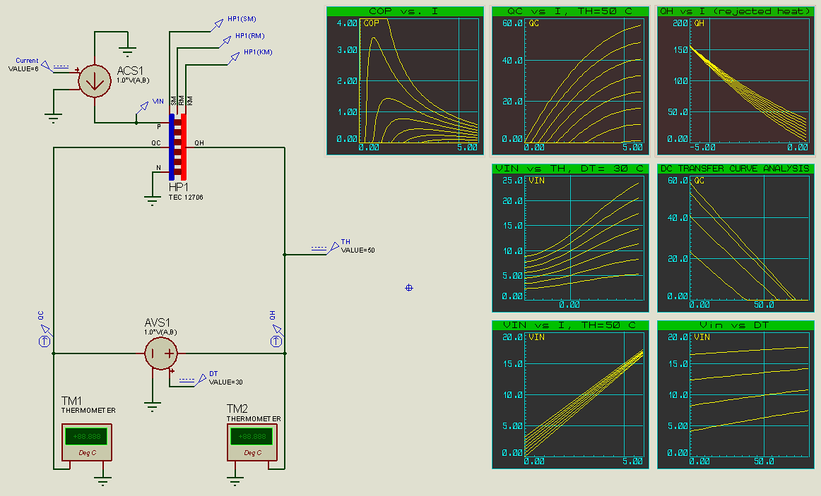 Peltier Performance Curves with Graph Based Simulation.
The Proteus file for analysing performance curves is linked below and can be evaluated with the demo software.
A demo copy of Proteus is required to open the .pdsprj file.
Case Study: Single Module Peltier Cooling System
Consider the case where we need to cool a component or something like dissipating a power in the neighbourhood of 12.5 Watts. We want cooling to 5°C from an ambient temperature of 30°C. We also have available a Peltier module of 71 elements (couples) and 6 Ampere as Imax.
With the following Proteus schematic we can estimate the thermal system performances:
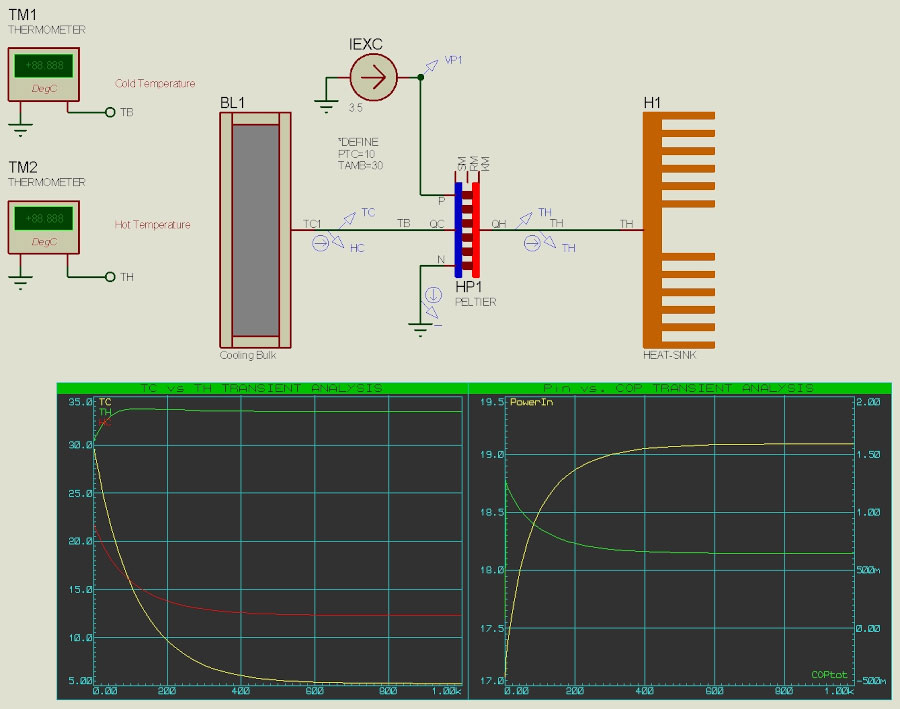 Peltier Cooling Sysmem Schematic.
The Proteus file for this schematic is available below and can be evaluated with the demo software.
A demo copy of Proteus is required to open the .pdsprj file.
The component BL1 and H1 represent the thermal models respectively for the component to be cooled and the heat sink used to improve the COP as discussed in the “Ways to Improve Peltier Efficiency” discussion above. Both of the component parameters are preloaded with relevant values.
In particular the BL1, Thermal Resistance (°C/W) is the value directly related to the heat flow (Qc) we need to remove from the component to be cooled. As we said we need to cool a component dissipating 12Watts of power, which implies we need to remove 12Watt of Qc heat flow. When we simulate thermal circuits heat flows are equivalent to currents and temperature equivalent to voltages. We therefore have:
Thermal Resistance = (30°C- 5°C)/Qc = 25/12.5= 2 °C/W
This is the value which has been set in the Thermal Resistance of the Edit Component dialogue.
Other values as the thermal capacity in J/K depends by the mass, the material and shape of the component/part/bulk to be cooled. The contact T Resistance (°C/W) is the typical value of a thin layer of silicon thermal compound used to improve the thermal contact between the Peltier cold side and the object to to be cooled.
We can now simulate the “TC vs TH TRANSIENT ANALYSIS” graph; the results are shown below:
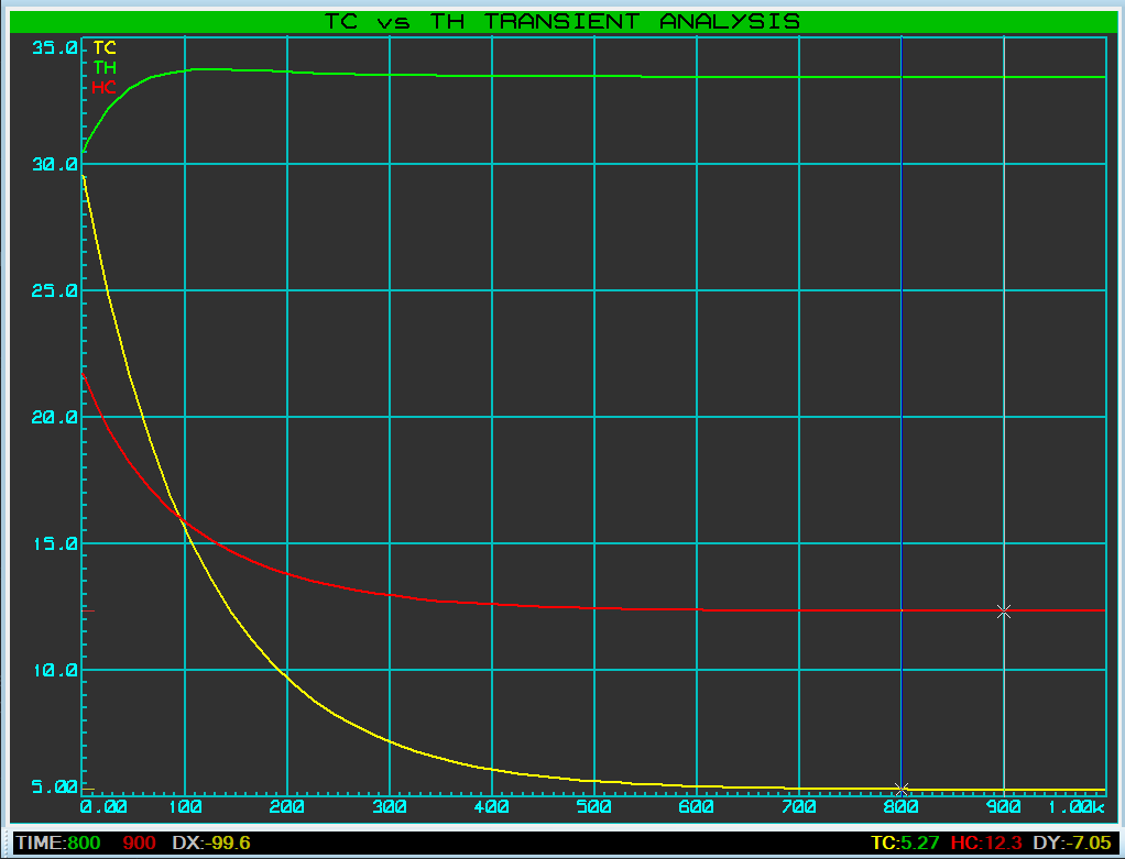 Tc vs Th Graph.
This simulation graph highlights quite a bit of significant information. With the selected Peltier module (71 couples and Imax = 6A), the calculated thermal resistance (including thermal losses) and Thermal Capacity (100 j/W) we get object cooling to 5°C after about 750 seconds (more than 12 minutes). However we’ve removed sufficient heat flow to achieve 10°C after just 200 seconds (3.3 minutes).
We can also check whether the IEXC = 3.5A mps is a consistent value or not to achieve the wanted Qc. We can use the performance curves as described in the chapter “How to get performance curves for a Peltier module” and estimate QC vs I curve. We need however to edit the HP1 componet (right click->edit component) and set the Number of Elements = 71 and Imax = 6A. Also we need to change the TH generator to 33.5 and DT generator to 28.5 (this produces a DT=5°C).
When we then simulate the performance graph Qc vs I we get:
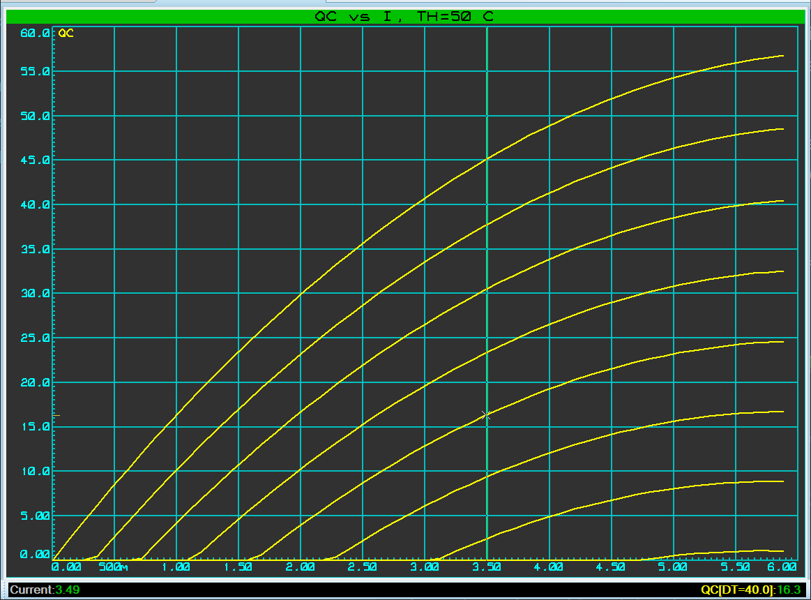 QC vs I Graph.
At the intersection of X axis =3.5(A) and the curve at DT=30 we get QC=11.7 which is sufficiently close to the power of 12.7 Watt we wanted to remove from the object to be cooled.
Another thing we can do is verify that the simulated COP value is consistent with the performance curve COP vs I.
By simulating the COP performance curves in the Peltier Performance Curves file and intercepting the X axis at 3.5(A) and the curve at DT=30 (°C) we get a COP value of 0.61, very close to the value simulated in this Peltier Cooling project.
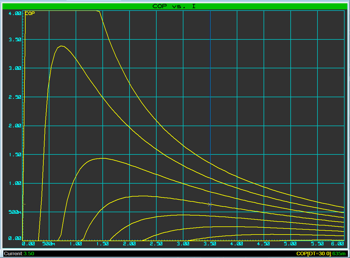 COP vs I Graph.
Proteus also offers a more complex application using Arduino, the standard PID libraries and Peltier model to simulate a simple temperature PID controller. The schematic is depicted here:
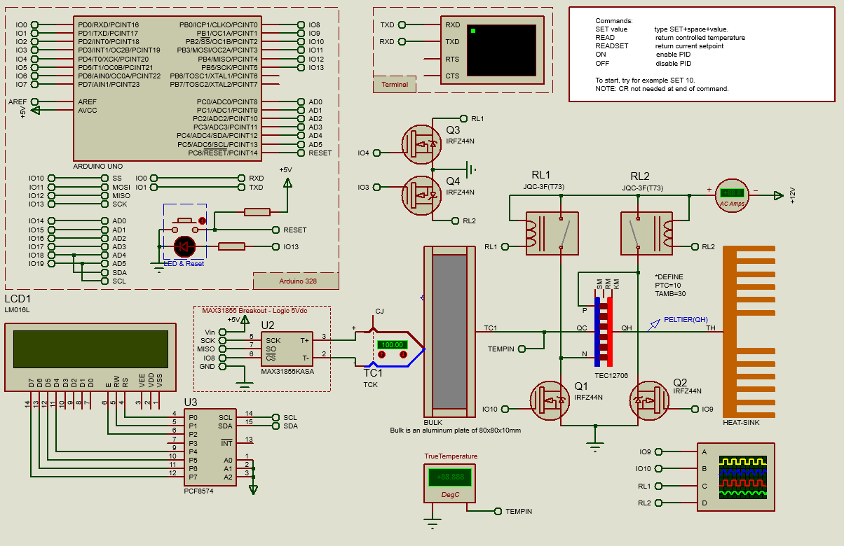 Arduino Peltier PID Schematic.
This sample schematic project is available for evaluation with the demo version of Proteus
Peltier Modules and Power Generation
The Peltier modules can be used in a “reversed” mode, albeit they are conceived as a solid state heating/cooling devices. If a differential temperature is applied across the two sides, then a voltage and current proportional to the number of elements, the Imax and the differential temperature itself, will be generated.
The Peltier module used as power generator components have many similarities with thermocouples. In fact, they exhibit a Seebeck coefficient in volt/°K exactly as thermocouples do. The equivalent voltage in open circuit will be:
V = S(volt/°K) * DT (°C)
and the current
I = (S * DT)/(Rm + Rl)
Where Rm is the electrical Peltier module resistance and Rl is the load resistance. The schematic below shows the concept:
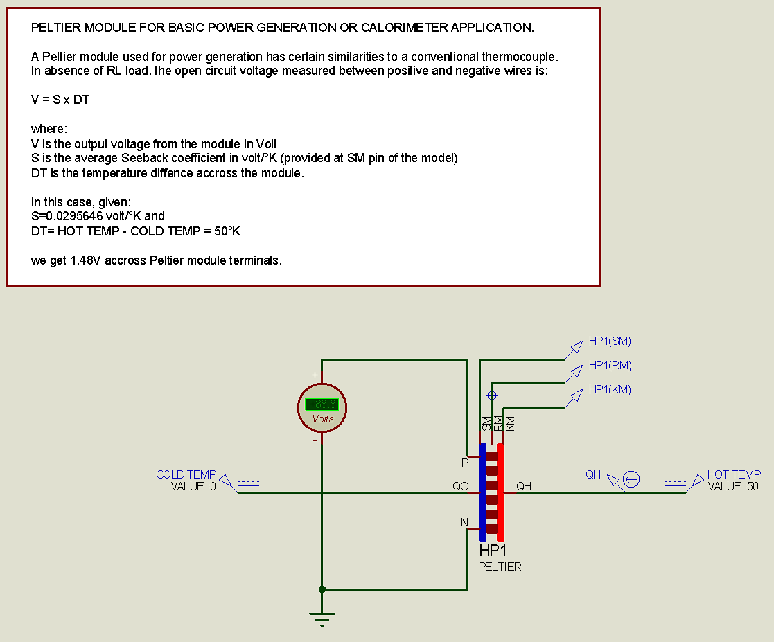 Peltier Power Generation Schematic.
Conclusion
The demanding need for eco-compatible systems and alternative energies made the Peltier modules assuming an increasingly importance. This article is intended to be a contribution to the basic understanding of these components.
This is a further example of how Proteus, with the help of suitable models, can simulate and predict the behaviours of many physical phenomena such as, in this case, the thermal performances of thermal systems based on Peltier thermoelectric modules.
Get our articles in your inbox
Never miss a blog article with our mailchimp emails