PID Control

Introduction

---

PID Control is an algorithm for controlling an output in order to maintain some process at a precise value. Some examples include:

• Controlling the rudder position on a ship in order to steer to a particular heading.
• Controlling the power provided to a heating element in order to maintain a particular temperature.
• Controlling the engine throttle in a car in order to maintain a particular speed (“cruise control”).
• Controlling the position of ailerons on an aircraft in order to maintain a particular rate of turn.
• Controlling the rate of chemicals being added to a stream of water in a water-treatment plant.

PID has three variables, namely the input, the output and the setpoint. The PID algorithm controls the output in order to get the input to match the setpoint.

For example, in the scenario of controlling a ship’s rudder in order to steer to a particular heading:

• Input is the compass or GPS heading.
• Setpoint is the desired heading.
• Output is the rudder angle.

The difference between the Input and the Setpoint is called the Error, and the PID algorithm aims to eliminate the error in the process. In order to understand why PID is needed, let’s first look at simpler methods of process control.

Bang-Bang Control

---

Bang-bang control is a digital form of control where the output is either completely on (maximum) or completely off (minimum), and nothing in between. This sort of control seems more intuitive when the output is also digital; such as a valve which is either completely open or closed, or an air-conditioner which can switch on or off. Using the example of an air-conditioner, the input would be provided by a temperature sensor and the setpoint would be the desired temperature to be maintained. The algorithm is simple:

If the measured temperature is above the setpoint then we turn the air-conditioner on, otherwise we switch it off.

For some applications this may work fine. For others however, there may be one or both of two problems which could be encountered:

1. Fast changing readings around the setpoint.

The first problem is that of relatively rapidly fluctuating readings around the setpoint. Imagine for example that the setpoint is 20°C. Depending on the air currents swirling around the room, or the stability of the temperature sensor, the reading may fluctuate between for example 20.1°C and 20.0°C; each time the temperature reading was just 0.1°C above the setpoint then the air-conditioner would switch on again, and as soon as the reading was 20.0°C again then it would switch off again. This could potentially happen very quickly, which would be both annoying to the people in the room, and possibly damaging to the air conditioner. . If there was both cooling and heating available we could imagine a scenario where the temperature was fluctuating between 19.9°C and 20.1°C, with both the aircon and heater switching on and off relatively rapidly – both working against each other and wasting energy.

The solution is to add some delay or buffer around the setpoint, and this is called hysteresis. A hysteresis of 2°C in our example would mean that once the temperature had reached 20°C and the aircon switched off, then the aircon wouldn’t switch on again until the temperature had risen to 22°C again. If there was heating available as well then the heating wouldn’t come on until the temperature had dropped to 18°C (but once on wouldn’t switch off again until the temperature had risen to 20°C).

2. Overshoot.

The second problem which may be encountered is that of overshoot. Overshoot is typical where there is a delay between when the output is commanded and when the result of that output command is measured by the input. Take the example of adding chemicals to a stream of water at a water-treatment plant: The chemicals take some time to dissolve into the water, and so we can only measure the result, perhaps the pH, a little way downstream of where the chemicals are added – i.e. there is some delay in the process. Let’s say that we start off with the pH being a little too low, so we open the valve to add an alkaline to the water in order to bring the pH up a bit; this starts working, but by the time we are reading pH neutral at the sensor, and close the valve, a flood of alkaline has already been added upstream and the sensor reading far overshoots neutral, and we start getting a very high pH reading; the system now reacts to the high pH reading by opening the valve to add an acid to the water in order to bring the pH down again – but by the time the effect of this reaches the sensor we have again overshot neutral and the reading goes too low again… The process repeats and the output continues to wobble around the setpoint – possibly oscillating further past the setpoint than the magnitude of the original error which triggered the corrective reaction.

If we look at the examples of controlling the rudder position of a ship or the engine throttle position in a car, then it is also more intuitively obvious that a better control system than the bang-bang one is needed – we don’t want to swing the rudder full right (starboard) or full left (port) if only a small correction in course is needed; or have the car accelerator oscillating between pedal-to-the-metal and completely off – we need something in between.

Proportional Control

---

Proportional control (the P in PID) does just what it says, and controls the output in proportion to the difference between the input and the setpoint (in proportion to the error). If the difference between the input and the setpoint is small then we only make a small adjustment to the output, and if the difference is large then we make a big adjustment to the output. If the ship is only slightly off-course then we only apply a slight turn on the rudder – we don’t turn it all the way as far as it will go. For some systems, proportional control may be all that is needed. For other systems however, the next type of problem is encountered:

Integral

---

When using proportional control, there will almost always be some level of steady-state error – meaning that the system doesn’t quite reach the setpoint, because the amount of proportional control near the setpoint is too small to overcome some bias which is affecting the system (perhaps a current or wind). In the image below, the process stabilises a bit below the setpoint.

The integral (I) part of PID looks at how long the system has been deviating from the setpoint and ramps up the output in order to overcome that deviation. If the cruise-control on a car was set to 60mph for example but the speed was stuck at 57mph using proportional control alone (due to air or other resistance), then the “integral” part of PID would over time ramp up the engine power to get the speed up the 60mph setting. Again, for some controllers PI control may be all that is required. PI alone however is prone to at least some overshoot and oscillation around the setpoint before settling, especially when there is a large intial difference between the setpoint and the input reading (such as at startup or when a large adjustment is made to the setpoint), since the integral part of the PID will accumulate all of the error during the transition period and thus become large (larger than needed), and without anything else to dampen that then the only thing which will reduce it again will be some accumulated error in the opposite direction. The D part of PID addresses this problem:

Derivative

---

The derivative (D in PID) element minimises or eliminates overshoot by easing / dampening the output depending on how quickly it is approaching the setpoint; if the input reading is moving very quickly towards the setpoint then the derivative part of PID will motivate to ease off on the output in order to minimise or eliminate overshoot. In mathematics, the derivative of a curve is the angle or gradient of that curve at a specific point – the rate-of-change – and that is what this term refers to. In the image below, the red line represents a steep gradient (which would result in a large D correction in the PID algorithm), and the blue line represents a shallow gradient (which would result in a small D correction in the PID algorithm).

Tuning

---

Each of the elements in the PID algorithm – the Proportional element, the Integral element and the Derivative element, can be tuned or weighted to give it a larger or smaller effect in the algorithm, and the correct values vary from application to application. PID tuning is a deep topic, the full depth of which is beyond the scope of this article, however having a good understanding of what each of the elements in the P, I and D does is a good starting point. Options include looking up some default values for the particular type of process, manual tuning, and simulation.

Manual tuning briefly involves tuning each of the P, I and D elements in order:

• First the I and D weights are set to zero, and the P weight is increased until the system begins to oscillate around the setpoint. The P weight is then set to half of this value.
• Next, the I weight is increased until any steady-state error is corrected quickly enough, but not so much that the system becomes unstable.
• Finally, the D weight is increased until any overshoot has been sufficiently dampened, but not so much that the system becomes sluggish to respond or even becomes unstable (which can happen especially if there is some noise in the input).

Digital Output Control with PID

---

Where the output controlled by the PID is digital, such as a relay or solenoid valve, techniques such as pulse-width modulation can be used to effectively convert the digital output into an analogue one. For more informaiton on pulse-with modulation, please see our PWM article. PWM frequency is chosen according to the application, and depending on the system additional constraints may be implemented such as only switching the output once the duty-cycle is above a certain level.

Here's an example of PID control for an oven using a PICCOLO microcontroller, simulating in Proteus VSM.

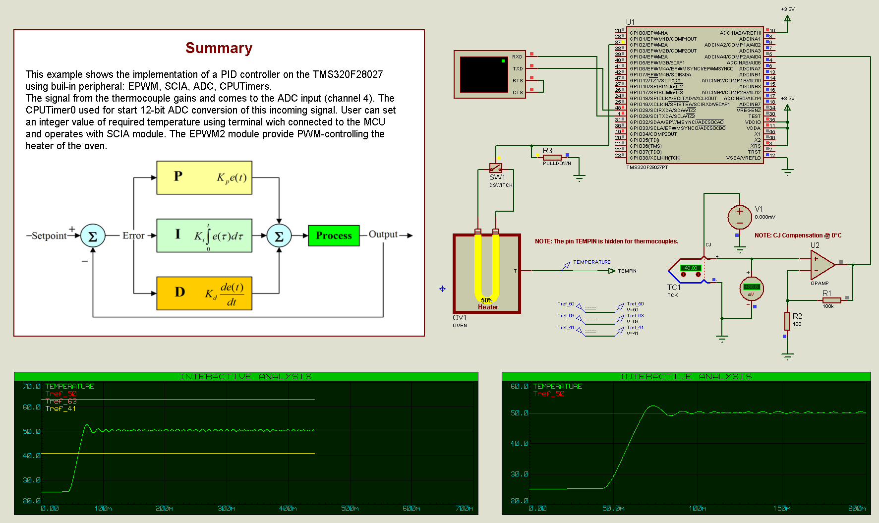
Head over to the Sample Design Browser to quickly find a set of ready-made embedded simulation sample projects that are included with the Proteus demo version.

All content Copyright Labcenter Electronics Ltd. 2024. Please acknowledge Labcenter copyright on any translation and provide a link to the source content on www.labcenter.com with any usage.